 Data validation, when used within the Excel framework, is basically a control function. In this excel tutorial I will show you how it prevents users from entering bad data into a particular cell. Most often, users inadvertently enter the information into the wrong cell, but if the cell is programmed with an excel drop down list, they will be required to choose the right information. Obviously, this feature adds credibility to a document, as there is less chance of error, and at the same time, information entered can be completed in an expeditious fashion. Creating a drop down list in Excel provides accuracy, efficiency and higher productivity through speed.
Create a Table
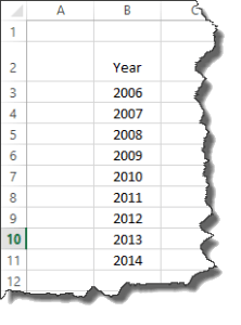
 Make a table by entering your title and parameters into a sheet in your workbook.
- Be sure that your title is in the cell right below the Letter Heading. Do not leave spaces between any cells.
- Your parameters will be entered in column fashion vertically, not by row horizontally.
- Now, name the table by clicking on any cell in the parameters and look for the Insert, click Table.
- Make sure your full list is highlighted, then click the Checkmark to include Headers.
 Make a table by entering your title and parameters into a sheet in your workbook.
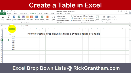

Create a Dynamic Range
The next step is to attach a named range to the table. The benefits of doing this is that it allows you to add items to your drop down list by simply appending the table. But Data Validation doesn’t like to attached directly to tables. So this intermediate step will solve the problem.
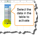
First you should select the data in the table to activate it. Just highlight all of the data in the column but be sure to NOT select the header. The data that you select will feed the syntax that is needed in later steps.
Then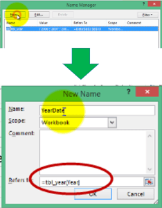 Select Name Manager, highlight your Table and Select “NEW”
Next, Select the Table from Step #1 and Select New
You will notice that the correct syntax is auto-filled. This is why it was important to only select the data in the table to activate before selecting the Name Manager

Assign Named Range to Data Validation List
Next you must create the drop down list and attach it to the Dynamic Range that you created in the previous step.
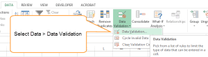 First, select Data > Data Validation
Then select “LIST” from the drop down box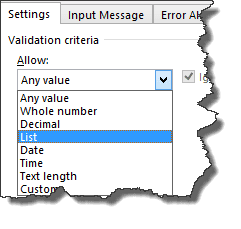
Now here is the COOL part. Enter the Named Range from Step #2 and everything will work perfectly. WOOT.

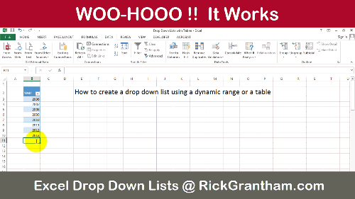
Test it — It Works
Add more data at the end of your original list and you will see that the items are auto-magically added to the drop down list. That’s AWESOME !!!

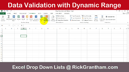
Drop Down using a Dynamic Range in Excel
Download the Excel Drop Down File

Download the file and follow along with the video.
Yours for free. 🙂
 Check out the rest of our Drop Down List Series
 Check out the rest of our Drop Down List Series
- Excel Drop Down List – 3 Types of Drop Down Lists – Includes PREMIUM content
- How to create Drop Down Lists in Excel – Using Dynamic Ranges
- Create a Dependent Drop Down List –
Well —- Whatta ya’ think? Got an extra twist to this that you think might help my readers? Got something to add? Don’t be shy. Leave a comment below and let me know what you think.
Also, if you think that a colleague might get some value out of this, feel free to hit one of those social sharing thing-a-ma-jigs. I’d appreciate it. As I tell my kids… sharing is caring 🙂
Until next time
Be A Champion
Rick Grantham
- The Comprehensive Guide to the Excel Ribbon: Making the Most of Your Data - January 31, 2023
- 51: Oz du Soleil & the Global Excel Summit 2021 - February 8, 2021
- 50: Randy Austin – Excel for Freelancers - January 22, 2021
