Random Sorted Order without Repeats Using Excel Formulas

There might be times when you need to shuffle a list of distinct items. It can be to run a simulation analysis, to pick a random sample for statistical analysis or to just have some fun. All you have to do is generate random integers between 1 and the size of your list. And then rearrange the list using the INDEX function. Simple, right? No, there’s a problem with this approach: random numbers could repeat!

As you would’ve guessed by now, we are here to present a solution which does NOT involve VBA. Excel MVP Jordan Goldmeier is here to ensure Excel fanatics sleep peacefully tonight.

So, let’s see what Jordan has in the bag for us.

1 – Numbering

The first step is to number your list of distinct items starting from 1. Let’s say we have a list of size 5.  Then you would number them from 1 to 5. This numbering will help us reorder the list towards the end. The image on the right illustrates this.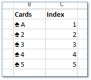

2 – Generating Random Numbers

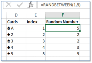
This is the fun step. Normally we would generate numbers between 1 and the size of your list using the RANDBETWEEN function. But that is where the repetition occurs, as shown in the image on the right.

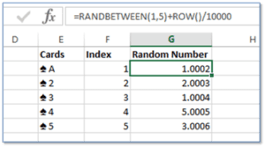
To avoid it, we will add a very small number to each random integer we generate. But these “small” numbers must change as the row number changes to make the overall sum unique.

The way to achieve this is to use the following formula:

=RANDBETWEEN(1, list_size) + ROW()/10000

ROW just returns the row number, which is obviously unique for each row. The division by 10,000 makes sure that this number is small. The overall result should look something like the image below.

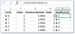
3 – Ranking In Excel

You may have observed that the random numbers are unique now. All we have to do is to rank them. We can use the formula RANK to rank the random numbers. Since the formula takes in the column array of random numbers, you can lock it by pressing F4 to copy the formula effortlessly. The image on the right illustrates this step.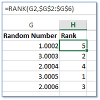

4 – The Final Step

This is where you get to reap the result of all your efforts. You can use the ranking to get your shuffled list using the INDEX function. The array would be your original list and the row number will be the rank in that column. Do not forget to lock the array reference to ease copying the formula. The overall result should look something like this:

Just one thing to note here: although 10,000 was selected randomly to add “small” numbers to the random numbers, you have to make sure whichever number you select is larger than your list size.

Get the download