This doesn’t have to be difficult.
It doesn’t have to be hard.
No need to stick your head under the covers.
There is no boogie-man coming to get you.
Doing “mathy” type things in Excel can actually go a long way in helping you run your business or team.
Quit Reacting So Much
It is common for Executives, Management, Small Business Owners, etc spend way too much reacting to data that they have no need to react to. This happens all the time. People are used to reacting, but not necessarily used to following a process of thinking through a problem.
Processes are designed to give specific outputs – within a range. You want to spend your time reacting to things that actually require your attention — not things that are just part of the normal fluctuations in your process.
My Rules for Using Standard Deviation
These are not written in stone. But rather some high-level things I take into consideration before deciding to use standard deviation.
- 30+ data points. – I try to make sure that there is enough data. The detailed reasoning for this is beyond the scope of this Excel tutorial, just know that you need enough data so that the formula makes sense. Different books will give you different sample sizes for this. 30+ is a good number for me. If you have too few data points, then the standard deviation tends to be very large to account for your small number of data points.
- Normal data – When we release a new blog post on Excel TV, traffic spikes for a day or so. If traffic multiplies by 5, then that skews the data… meaning that the mean (average) is wildly different from the median (half higher, half lower than a number). One or two high numbers are skewing the curve. This also happens in home prices where a few mansions throw off the average. Look to use standard deviations on data that is “normal”. By “normal” I mean that it resembles a bell-curve.
Setting up the Formula

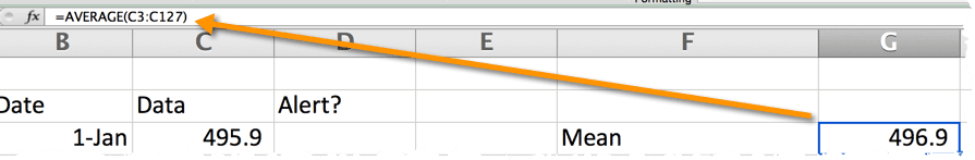
Calculate the Mean
This is simply calculating the average of your data points. Realize that standard deviations are based on the mean, so this must be your starting point. In the example, our data points reside in cells C3:C127. So the Mean would be…
=AVERAGE(C3:C127)
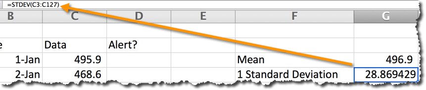
 Calculate One Standard Deviation

Use the formula STDEV() for this. Within the parenthesis you will enter the range for the data points that you used to calculate the MEAN in step 1. So one standard deviation would be…
=STDEV(c3:C127)
Hold up… wait a minute
Before we move any further, we should discuss the difference between 1, 2, and 3 standard deviations.
In a normal distribution a certain number of data points would typically expected to be included within 1, 2, or 3 standard deviations from the mean.
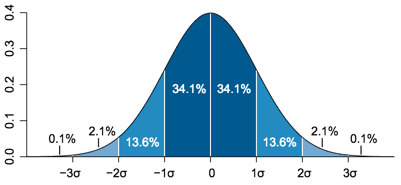
- 1 standard deviation encompasses 34.1% on either side of the mean. Which is 68.27% of data points in perfectly normal data.
- 2 standard deviations = 95.45%
- 3 standard deviations = 99.73%
- 4 standard deviations = 99.994%
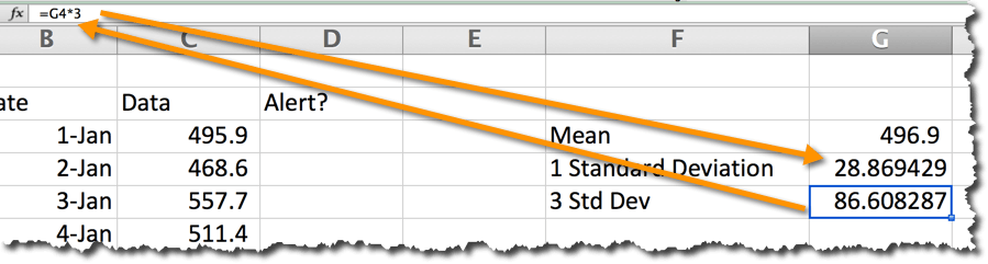
 Calculate 3 Standard Deviations

Take the one standard deviation output and multiply it by 3.
 Set Your Control Limits

In the example, I use the terms UCL and LCL. These stand for “Upper Control Limit” and “Lower Control Limit”. If you were creating a Control Chart (like in Six Sigma) these limits would be the lines on the chart that would tell you when your process is out of control.

In the example, I set this for 3 standard deviations from the mean, so that I am only reacting 0.27% of the time. Reset this for a different number of standard deviations based on your business needs.
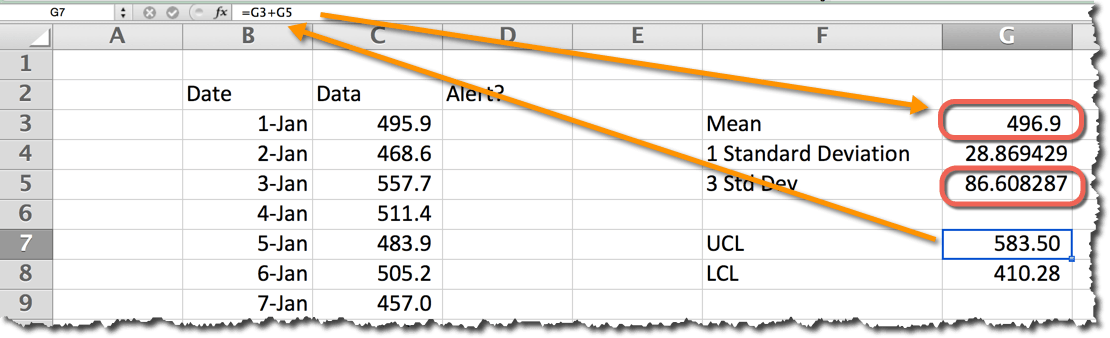
For the UCL – Add the Mean plus the standard deviations. In this instance I am using 3 standard deviations, so 496.9+86.6 = 583.50
For the LCL – Subtract the standard deviations from the mean For the 3 st dev example it is 496.9-86.6 = 410.3
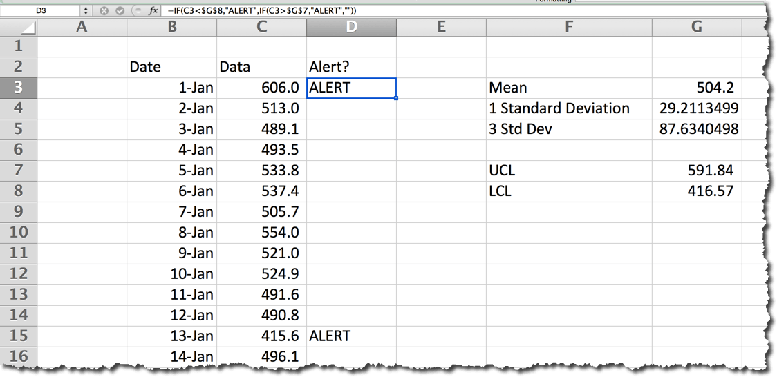
Set Alerts
Now bring it all together with a nested IF statement. The statement is stating that if the data is lower than the LCL or Higher than the UCL – then “ALERT”, else null “”.
Definitely could have used conditional formatting or something more exotic here, but the point is not about this formula, but rather that you are now using alerts in conjunction with Standard Deviations to more accurately pinpoint data that requires your attention.
Download the Sample
[thrive_link color=’teal’ link=’https://excel.tv/wp-content/uploads/Standard-Deviation1.xlsx’ target=’_blank’ size=’small’ align=’aligncenter’]Download the File[/thrive_link]
What’s Next?
The stats show that 40% of you are repeat visitors to the website. So you might as well just join our mailing list and get alerted when we release new content.
First timer? Then tell your colleagues about us and hit one of those social sharing thing-a-ma-jigs.
Attribution: “Standard deviation diagram” by Mwtoews. Licensed under CC BY 2.5 via Wikimedia Commons – http://commons.wikimedia.org/wiki/File:Standard_deviation_diagram.svg#/media/File:Standard_deviation_diagram.svg
- The Comprehensive Guide to the Excel Ribbon: Making the Most of Your Data - January 31, 2023
- 51: Oz du Soleil & the Global Excel Summit 2021 - February 8, 2021
- 50: Randy Austin – Excel for Freelancers - January 22, 2021

Very nice )
Thanks Dmitry 🙂
Great, clean & easy!
Thanks Stramilov
This is a great tutorial for calculating standard deviation in excel.