Updating spreadsheets can be a pain, especially when you have to change all the Data Validation dropdown menus manually. Of course, you may use a complicated mix of INDIRECT and ROW formulas to achieve a dynamic dropdown list. But there is a much better solution. And that is exactly what Zack Barresse is here to present.
Let’s get started!
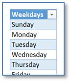
1 – Excel Table
Convert the list of values you need in your dropdown menu into an Excel table. You can go into DESIGN and rename the table under the ‘Properties’ section. We have given it the name ‘Table_Name’.
2 – From Excel Table to Named Range
Press CTRL + F3 or go to FORMULAS > Name Manager and select New. This is just to name our newly created Excel table.
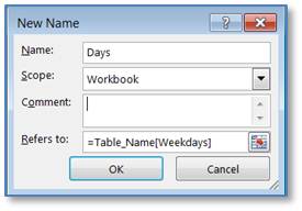
In the ‘Name’ field, assign a unique name for the range. Hence, ‘Table_Name’ cannot be used. We have used ‘Days’ here. In the ‘Refers to’ field, use the syntax below. When done, click on OK.
< table name >[< field name >]
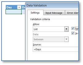
3 – Data Validation List
Now select the cell you want to apply the dynamic dropdown menu to and go to DATA > Data Validation. Select ‘List’ from field ‘Allow’ and, within the ‘Source’ field, write the new name of the table with ‘=’ as a prefix. Now click OK and you’re are done.
4 – Play!
You can see that the dropdown menu will get updated automatically whenever you will make a change to your table ‘Table_Name’. This includes increasing the items in the list, reducing the size of the list or modifying the individual values.
What’s next?
Implement it! Test it on random spreadsheets and, once you’re comfortable, use it on the files you update quite frequently. Cumulatively, it can potentially save you a lot of time.
Do not forget to share this technique with your friends or colleagues. And write to us with your comments and suggestions below.
- SSSVEDA DAY 7 – Every Team Needs Someone Who Understands Data - February 18, 2018
- SSSVEDA DAY 5 – When Data Analysis is Wrong - October 31, 2017
- SSSVEDA DAY 4 – Sharing the Excel Knowledge - July 18, 2017

Very impressive