Cleaning Name Suffixes with Array Formulas

Have you ever wondered how to sort lists using 2^nd word in each cell? Sounds a bit tricky, doesn’t it?

But don’t you worry, Oz du Soleil is here to help. He uses a neat trick to sort out full names by the last names. The approach is interesting and can be modified to achieve many similar task.

Now, let’s explore

Create a List of Suffixes

Some last names may be followed by suffixes such as “Jr.” or “PhD”. It is important to make sure that EXCEL does not pick them up as the last names of an individual. So, the first (and the only manual step) is to create a list of suffixes present in the list of names you want to sort.

Note that suffixes are those which follow the last names with a space in between!

Create a Table of Suffixes

Now, go to Insert > Table and select the list and two more columns on its right.

Let’s name the columns from left to right: New Suffix, Sfx with Space and Count Characters.

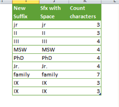
Now insert the formula =” “&[@[New Suffix]] in the 2^nd column of the table and =LEN([@[Sfx with Space]]) in the 3^rd column.

You should be able to see that the column titles correspond with what these formulae are doing.

Detecting a Suffix

Now, create a 6 column table (Insert > Table) with your original data on names in the leftmost column. The columns should be named from left to right as follows: Original Data, Test 1, Count Spaces, Replace, Delimiter and Result.

Go to first cell in Test 1 column. Now apply the formula =OR(RIGHT(x,y)=z) . x, y and z not to be typed! These are tasks to do.

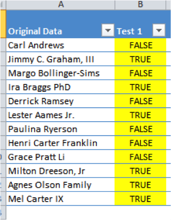
x is selecting the left cell.

y is selecting the Count Characters column from your suffixes table (without the header).

z is selecting the Sfx with Space column from your suffixes table (without the header).

Once you’re done putting in the formula, press Ctrl+Shift+Enter. This should give you an output which looks like the picture on the right.

Getting to the Last Names

It’s time to speed things up now!

In the Count Spaces column, first cell, enter the following formula:

=LEN([@[Original Data]])-LEN(SUBSTITUTE([@[Original Data]],” “,””))

And press Ctrl+Shift+Enter.

Enter the following formulae using the same method as well:

Replace
=IF([@[Test 1]]=TRUE,SUBSTITUTE([@[Original Data]],” “,”^”,[@[Count Spaces]]-1),SUBSTITUTE([@[Original Data]],” “,”^”,[@[Count Spaces]]))

Delimiter
=FIND(“^”,[@Replace],1)

Result
=RIGHT([@Replace],LEN([@Replace])-[@Delimiter])

And you are done! You should now have the last names in the rightmost column now.

Now Sort Them!

Get the download

[button size=”large” url=”https://excel.tv/wp-content/uploads/Name-Suffixes-and-Array-Formula.xlsx” text=”Click to download the file that Oz used” target=”” color=”orange” ]

What’s Next?

Use this the next time you need to do some tricky sorting.  Share it.

• Author
• Recent Posts

Jamani Arsalan

I am a healthcare consultant, currently based in Middle East, at an international professional services firm. My work largely revolves around project management, and statistical analysis. And my professional interests include developing my knowledge within the discipline of health analytics.

Latest posts by Jamani Arsalan (see all)

• SSSVEDA DAY 7 – Every Team Needs Someone Who Understands Data - February 18, 2018
• SSSVEDA DAY 5 – When Data Analysis is Wrong - October 31, 2017
• SSSVEDA DAY 4 – Sharing the Excel Knowledge - July 18, 2017