
What if there is a way to define new formulas in Excel without using VBA? One would be very skeptical of any such claims. But, believe it or not, it is true. Think about how easy such a technique would make your life. Not only would it allow you save a lot of time, the technique is also very handy in simplifying or restricting complex formulas to stop your audience from making blunders while using your files. Moreover, it’s extremely simple to do!
Our very own Excel expert Szilvia Juhasz has uncovered this life-saving functionality for the fans, giving us all the more reasons to thank her.
So, let’s see what the technique actually is.
1 – Name Manager
We all are aware of how we can name ranges using the Name Manager. Let’s review it:
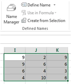 Select a range (or even a cell) with some data.
- Go to the Formulas tab, and click on Name Manager.
- Now click “New”.
- Type in any name, without spaces, for the range. We will use the name “ABC”.
- Now click “OK” and then click “Close”.
- In any cell outside the range ABC, type a sensible formula which can take ABC as an input. E.g., =PRODUCT(ABC).
- And you would see that it works perfectly well.
2 – Advantages of Named Ranges
There are 2 apparent advantages of using named ranges.
- We do not have to worry about selecting the range (especially if it is big) repeatedly and carefully. It only has to be done once, followed by naming it.
- If our workbook has many sheets, switching between sheets again and again to select different ranges can be a pain. Named ranges eases the process dramatically.
Also, if we give meaningful names to our ranges, worries about getting confused or memorizing the names go out the window.
3 – The Trick
The trick uses the Name Manager and some ingenuity. Let’s take an example: we have the formula TODAY() in Excel which returns today’s date. But we do not have a corresponding equivalent for yesterday, or even tomorrow for that matter. Well, with this trick, we do.
 Go to the Name Manager and click “New”.
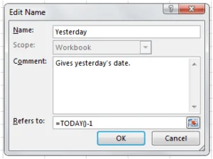
- In the ‘Name’ box, type the name to be given to the function. It will be “Yesterday” for the sake of this example.
- Now, in the ‘Refers to’ box, type the formula, which would be “=TODAY()-1” in this case.
- We can write any comments explaining the formula if we wish.
- Now click “OK” and then click “Close”.
4 – The Test
Go to any cell and type “=Yesterday”. And, there you have it!
Note that you do not need any parentheses in this case. Also, set the cell to any date format for it to appear like we would want.
What’s next?
Try it out! Now try it some more. Let’s make our lives simpler. And, share, share, share! Help the knowledge of your friends and colleagues grow.
Also, do comment below about any creative uses of this technique you might have come across.

Comments (3)
Historical comments preserved from the WordPress archive. Commenting is no longer active.
Very interesting! Can you imagine any ways to hack in a function parameter? Inquiring minds want to know!
Hi Mike. Yes! One could imagine hacking in function parameters. You could build a UDF using VBA, then use said UDF name in your drop down list. Or, you can use an existing Excel function that pulls argument values from cells on the worksheet, as demonstrated here: https://www.youtube.com/watch?v=G22rA-3PCio
Here’s a good one, which you can give the name SHEETNAME, or (my preference) CURRENTSHEETNAME:
=MID(CELL(“filename”),FIND(“]”,CELL(“filename”))+1,31)
You have to enter this PRECISELY the way it appears above, so copy/paste it folks. Also NB: “filename” is NOT a placeholder! it is to be typed as shown or this will not work.
You will almost certainly need to Save your workbook BEFORE you add this function to it; I’ve only ever typed (or pasted) this into workbooks which had already been saved.