
Isn’t it just frustrating to receive a copy-paste summary table that requires analysis? Yes, we’d rather have the data source, which we can turn into a pivot table and analyze to our hearts content. Well, the world isn’t perfect, but Ken Puls has a trick up his sleeve that can potentially save us from tons of manual work.
Let’s make that data pivot-ready!
1 – Importing Data
Let’s say that the Excel table you want to “unpivot” looks something like the image below.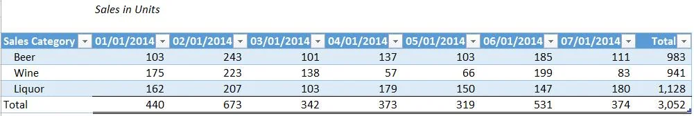
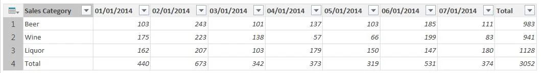
Analyzing this is difficult since it cannot be turned into a pivot table (just yet!). On your Excel sheet, select this table containing the data. Now go to POWER QUERY and click on ‘From Table’. Check the box as appropriate for your selection and click OK. The data will be imported into Query Editor and would look something like this.
2 – Data Cleansing
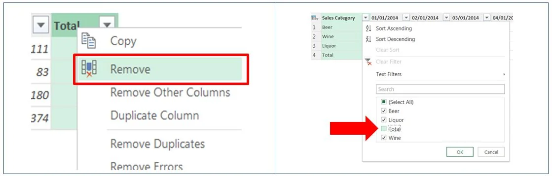
There are two simple steps to do at this stage before the magic can happen.
- Remove the “Total” column, and
- Filter out the “Total” row.
3 – The Magic
Select the column with the labels. Now go to Transform > Unpivot Columns > Unpivot Other Columns. And done! You should now have columnar data that can be pivoted easily. You can do the following improvements to the data table: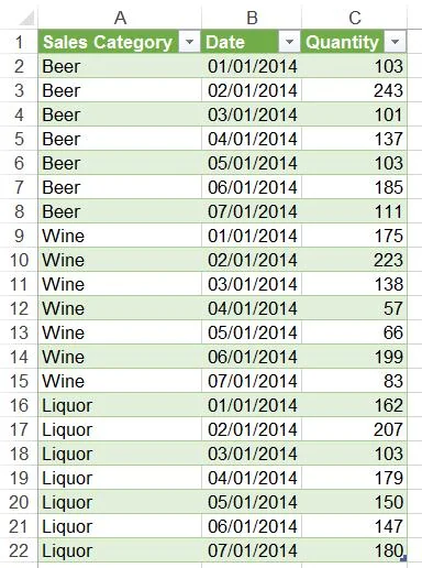
- Right-click on any column heading and select Rename.
- Select the date column and go to Home > Data Type > Date from the dropdown menu.
- Under ‘Properties’ from right-hand side panel, you can also change the table name.
Now press ‘Apply & Close’ or ‘Close & Load’ under the Home tab in your Query Editor. And the data is ready to use and will resemble the image on the right. You can pivot it and get to the exact same table you started with. Or you can come up with other pivot tables that might be more meaningful to you.
4 – Some More Magic
Let’s say the initial data summary got updated with more products and more columns, as depicted in the image below.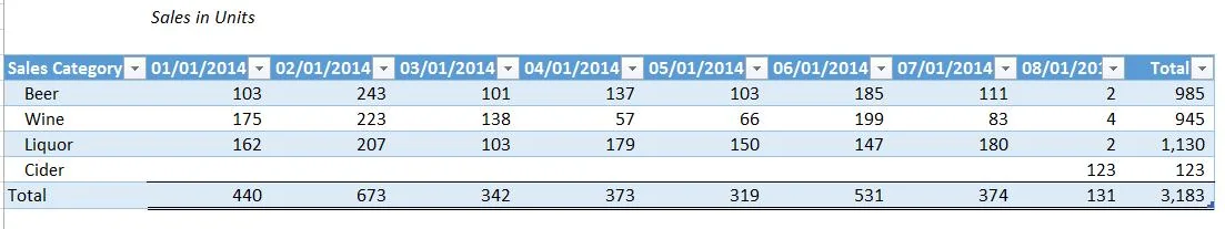
What should be done now? It would be a headache to have to repeat all of the steps explained above each time this our summary data gets updated. Well, you don’t have to. Just right-click on the output from Query Editor (the green table) and click ‘Refresh’. Done!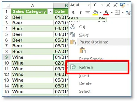
Similarly, you can also “refresh” your pivot tables connected to this table and they will be updated too.
5 – Extras
As an extra, Ken Puls shares with us a way to pull data (from our sources) faster. Under the POWER QUERY tab, click on ‘Fast Combine’ from Workbook Settings section of the ribbon and enable it. For Excel 2013, go to POWER QUERY and then click on ‘Options’ from Settings part of the ribbon and check ‘Fast Data Load’. Now you can load data by suppressing information or security settings and all alerts / notifications pertaining to them.
What’s next?
Oz loved the trick! And so did others. And, surely, you will too. Try it out now and see how it melts away some of your frustration in dealing with tabular data. And share with us your thoughts and experiences in the comments section below.
