Excel FILTER Function: Complete Guide

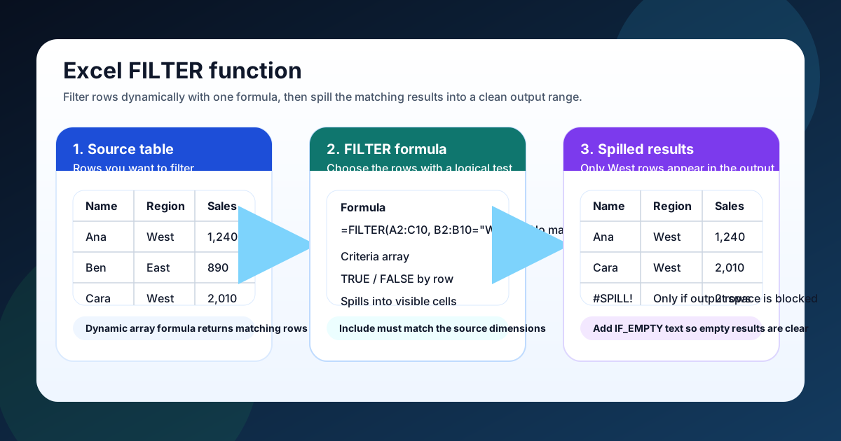
Short answer: the Excel FILTER function returns only the rows that meet a condition, and it does it as a dynamic array. If you want one formula to show a live subset of your data, FILTER is the cleanest choice. If you only need a single matched value, use Excel XLOOKUP instead.

FILTER is one of those formulas that feels simple once you have seen it work. You give Excel a source range, a logical test, and an optional fallback for empty results. Excel then spills the matching rows into nearby cells and keeps the output live as the source data changes.

That makes FILTER ideal for dashboards, working lists, customer slices, and any report where you want the row set to update automatically. It is also a better fit than AutoFilter when you need the filtered result to behave like a formula output rather than a manual UI filter.

What the FILTER function does

FILTER returns the rows or columns from a range that meet a logical test. In practice, that means you can point at a table and ask Excel to return only the matching records instead of hiding anything manually. The result is dynamic, formula-driven, and easy to reuse.

I like to think of FILTER as a formula that performs the same decision you would make with AutoFilter, but then hands the result back to the worksheet as an output range. That difference matters. AutoFilter changes what you see in place. FILTER creates a separate result set you can reference, format, sort, or feed into another formula.

Microsoft’s documentation also makes the structure clear: FILTER takes an array, an include argument, and an optional if_empty argument. The include argument must produce a TRUE/FALSE result for each row or column in the source data. If the test fails for every record, the if_empty message gives you a graceful fallback instead of a blank-looking failure.

Sourced stat block

• Microsoft documents 3 arguments for FILTER: array, include, and optional if_empty.
• The include argument must evaluate to a Boolean array that matches the source dimensions.
• FILTER spills its results into adjacent cells automatically, so the output can grow or shrink as the data changes.

Source: Microsoft FILTER function docs and Microsoft’s dynamic array behavior guidance.

That spill behavior is the real payoff. Instead of copying formulas down a helper column, you define the logic once and let Excel manage the output. If the source data changes tomorrow, the filtered list updates too.

FILTER syntax and the basic setup

The standard pattern is =FILTER(array, include, [if_empty]). The array is the range you want to return. The include argument is the logical test. The optional if_empty argument is the text or value to show when nothing matches. Once you understand that structure, the formula stops feeling mysterious.

A simple example looks like this:

=FILTER(A2:C10, B2:B10="West", "No matching rows")

In that formula, A2:C10 is the source data, B2:B10="West" is the include test, and "No matching rows" is the fallback. If the Region column contains West in row 2 and row 7, FILTER returns those rows from the full table.

A few setup rules make FILTER easier to trust:

• The include range must line up with the source range.
• Use the same number of rows for row-based filtering.
• Wrap text values in quotes.
• Use a cell reference when the criteria should be editable.

If the logic feels too dense, start with one literal condition first. For example, test B2:B10="West" on its own before you combine it with sales thresholds, dates, or text searches. That keeps debugging short and makes mistakes obvious.

How to use FILTER with one condition

For one condition, FILTER is straightforward: define the source, define the include test, and supply a fallback if you want a clean message when nothing matches. That one-condition version is usually the best place to start because it proves the spill range and the data shape before you add complexity.

Suppose column B contains regions and you want only the West rows. This formula returns every West record from the table:

=FILTER(A2:D100, B2:B100="West", "No matching rows")

You can also make the condition editable by placing the region in a cell:

=FILTER(A2:D100, B2:B100=F1, "No matching rows")

That is a better pattern for dashboards and report templates because it lets the viewer change the filter without editing the formula itself. If F1 says West, the spill shows West rows. If F1 says East, the spill updates instantly.

This is also where FILTER starts to beat manual filtering for repeatable work. With AutoFilter, you still have to click the dropdowns and set the criteria. With FILTER, the criteria lives in the worksheet and can be reused, copied, or wrapped inside a larger model.

A one-condition FILTER is especially useful when paired with summary formulas. For example, you can feed the spill result into COUNTA, ROWS, SORT, or a chart source. That turns a simple filter into a live report component.

How to use FILTER with multiple criteria

Multiple criteria are where FILTER becomes much more powerful. For AND logic, multiply the conditions together. For OR logic, add the conditions together. Excel treats TRUE as 1 and FALSE as 0, so boolean arithmetic becomes an elegant way to combine tests without helper columns.

Here is an AND example that keeps only West rows with sales greater than 1000:

=FILTER(A2:D100, (B2:B100="West")*(D2:D100>1000), "No matching rows")

Both tests must be TRUE for the row to survive. If either condition fails, the multiplication returns 0 and FILTER excludes the row.

Here is an OR example that keeps West or East rows:

=FILTER(A2:D100, (B2:B100="West")+(B2:B100="East"), "No matching rows")

Either test can be TRUE for the row to survive. That pattern is handy when you want a broader slice without adding extra helper columns or complex nested logic.

You can extend the same idea to dates, text searches, and numeric bands. For example:

=FILTER(A2:F100, (C2:C100>=DATE(2026,1,1))*(C2:C100<=DATE(2026,3,31)), "No matching rows")

That formula filters to a date window. In another model, you might use ISNUMBER(SEARCH("car",E2:E100)) to find rows whose notes contain a keyword. The point is the same: build a boolean array, combine it carefully, and let FILTER spill the matches.

If you are coming from COUNTIF or COUNTIFS, this pattern will feel familiar. The difference is that FILTER returns the actual rows, not just the count. That makes it much more useful for downstream analysis and display.

FILTER vs AutoFilter

FILTER and AutoFilter solve related problems, but they are not the same tool. AutoFilter is a worksheet interface feature. It hides rows in place. FILTER is a formula. It returns matching rows into a spill range that behaves like ordinary worksheet output.

That difference is important in real work. Use AutoFilter when you want a human to click around and inspect a list directly. Use FILTER when you want another formula, a dashboard, or a report to consume the filtered rows automatically.

I usually choose FILTER when I want the result to be visible outside the source table. For example, I might build a summary sheet where the user picks a region in cell F1, and the filtered results appear in a separate area. That setup is cleaner than hiding rows inside the raw data sheet.

AutoFilter still has a place, especially for quick manual review. But if you need a live, formula-driven result set, FILTER is the better fit. It is easier to audit, easier to reuse, and easier to combine with functions like SORT, UNIQUE, or INDEX.

For example, if you only need one matching value back, FILTER is overkill. A lookup formula is better. See Excel XLOOKUP for the one-value case. If you need to sum a filtered list rather than return the rows, the right companion page is Excel SUM Formula for Filtered Cells.

Common FILTER mistakes and how to fix them

Most FILTER problems come from shape mismatches, empty spill ranges, or unsupported Excel versions. The formula itself is usually fine; the data or destination is what causes the headache, and the fix is usually a quick shape check, a cleared spill area, or a simpler include test.

Here are the issues I see most often:

1. The include range does not match the source range. If the source has 100 rows, the include test needs 100 rows too.
2. The spill range is blocked. Existing values, merged cells, or tables can stop the output and trigger #SPILL!.
3. Text and numbers are mixed incorrectly. A numeric test written as text can quietly fail.
4. The workbook is not using a dynamic-array version of Excel. FILTER is not available in every legacy installation.
5. The logic is wrapped incorrectly. AND/OR logic inside FILTER should usually be built with multiplication or addition, not with the AND() or OR() functions.

A quick troubleshooting sequence helps:

• Check that the source range and include range are the same size.
• Clear the cells where the spill result should appear.
• Test one condition at a time.
• Replace any complicated include formula with a literal TRUE/FALSE test for debugging.
• Add the if_empty text so an empty result is obvious.

If the formula still fails, simplify the sheet layout. Move the output away from the source table and test again. That often reveals a hidden block or formatting issue in seconds.

Practical ways to use FILTER in real spreadsheets

FILTER becomes far more useful when you treat it as a building block instead of a one-off formula. A filtered spill can feed charts, summaries, data validation, or downstream formulas. That is where it earns its place in a workbook.

One common use is a live report slice. Put the source data on one sheet, put a control cell on another sheet, and let FILTER return the matching rows into a report area. The report updates when the control cell changes, so the workbook feels interactive without any VBA.

Another strong use case is a working queue. If you track tasks by owner, status, or due date, FILTER can surface only the rows that matter right now. That gives a cleaner view than manually hiding rows, and it avoids accidental edits to the source table.

You can also use FILTER as a pre-step before other formulas. For example, you might spill a subset into a helper area and then run SORT, UNIQUE, or COUNTA against that result. That pattern keeps your workbook modular and easier to maintain.

If you are building a formula chain, I usually recommend this order: filter first, then sort, then summarize. That mirrors how people think about the data. First find the rows. Then arrange them. Then analyze them.

When FILTER is the right choice and when it is not

FILTER is the right choice when you need a live subset of rows and you want Excel to manage the output automatically. It is especially strong in dashboards, live reports, and reusable templates. It is less useful when you only need one value or when the workbook layout cannot tolerate spill output.

Use FILTER when:

• You want every matching row, not just a single match.
• You need a formula-driven result that updates automatically.
• You want to feed the output into another formula or visual.
• You prefer worksheet logic over manual filtering.

Do not reach for FILTER when:

• You only need one returned value. Use Excel XLOOKUP instead.
• The spill range is too constrained.
• You are working in an older Excel version without dynamic arrays.
• You need a one-time manual inspection of a sheet.

That is the simplest way to think about it. FILTER is a live row selector, not a lookup and not a visible-cell aggregator. Once you keep that distinction in mind, the formula becomes easy to place in the right part of the workbook.

Quick recap

FILTER returns matching rows as a dynamic array. Build the include test carefully, combine multiple criteria with boolean arithmetic, and clear space for the spill output. If you need one row, use XLOOKUP. If you need a total for visible filtered cells, use the filtered-cell sum guide. If you need manual hiding in the sheet interface, AutoFilter is still fine.

FAQ

How do I use the FILTER function in Excel?

Use =FILTER(array, include, [if_empty]). The array is the data you want returned, the include argument is your logical test, and the optional if_empty argument gives Excel a fallback message when nothing matches. Those three pieces cover almost every real-world FILTER question, from one-condition slices to spill errors.

How do I use FILTER with multiple criteria?

Use multiplication for AND logic and addition for OR logic. For example, =FILTER(A2:C10,(B2:B10="West")*(C2:C10>1000),"No match") keeps rows that satisfy both tests.

Why does FILTER return #SPILL! in Excel?

#SPILL! usually means the destination cells are blocked. Clear the output area, remove merged cells if needed, and make sure the spill range is not inside a layout that leaves no room for the results.

What is the difference between FILTER and AutoFilter?

AutoFilter hides rows in place. FILTER returns the matching rows into a separate spill range. AutoFilter is great for manual review, while FILTER is better for formula-driven reports.

When should I use FILTER instead of XLOOKUP?

Use FILTER when you want every matching row back. Use XLOOKUP when you only need a single matching value. If you are comparing the two approaches, the Excel XLOOKUP guide is the better companion.