
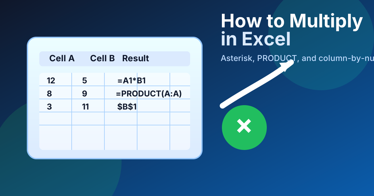
=A1*B1 is the Excel multiplication formula for multiplying two cells. Start with =, point to the first value, type the asterisk operator, point to the second value, and press Enter. That single pattern handles most row-by-row calculations, from quantity times price to hours times rate.
When the job gets larger, the formula changes by purpose rather than by difficulty. Use =A2*$B$1 when every row needs the same fixed multiplier. Use =PRODUCT(A1:A5) when you want to multiply a range or several arguments without building a long chain of asterisks. The best Excel multiplication formula is the one that stays readable after you copy it.
If you already know Excel SUM Formula and Excel Subtraction Formula, multiplication follows the same reference logic with a different operator. Addition, subtraction, and multiplication all reward the same habits: keep inputs visible, lock constants deliberately, and audit the formula before filling it through a worksheet.
By the numbers: Microsoft’s Excel specifications for Excel 2024 and Microsoft 365 list a worksheet limit of 1,048,576 rows by 16,384 columns, with 255 arguments allowed in a function. That scale is exactly why copied multiplication formulas need locked references and spot checks. Source: Microsoft Support — Excel specifications and limits.
Key takeaways
Use =A1*B1 for the basic Excel multiplication formula, =A2*$B$1 when one multiplier must stay fixed, and PRODUCT when the inputs form a range. The main decision is not mathematical; it is whether the formula will remain clear when copied, audited, or handed to someone else.
- Use the asterisk (
*) for quick row-by-row multiplication. - Use
PRODUCTwhen you want to multiply a range or several arguments at once. - Lock a constant with
$when you need to multiply a whole column by one fixed number. - Convert text numbers before troubleshooting, because one text cell can break a formula chain.
- If you are moving from addition or subtraction, the same reference habits still apply; only the operator changes.
How do you multiply cells in Excel?
To multiply cells in Excel, type an equals sign, click the first cell, add an asterisk, and click the second cell. The basic pattern is =A1*B1, and it is the quickest way to multiply two values in a single row. When I need a plain result fast, this is the formula I use first.
Here is the shortest path:
- Click the result cell.
- Type
=. - Click the first cell reference.
- Type
*. - Click the second cell reference.
- Press Enter.
For example, if A2 contains 12 and B2 contains 5, the formula =A2*B2 returns 60.
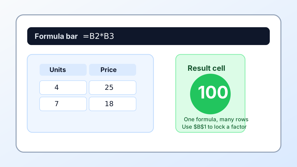
A couple of habits make this simpler to copy later. First, keep the formula in the same row as the data so the references are easy to read. Second, use relative references unless you know one side must stay fixed. That way, when you drag the formula down, Excel automatically adjusts the row numbers for you.
A common pattern is line-item pricing. Suppose column A holds quantities and column B holds unit prices. In C2, write =A2*B2. Then fill the formula down. Every row multiplies its own quantity by its own price, which is exactly what most invoice and budget tables need.
If you are new to formulas, the idea is identical to subtraction or addition: the cell references matter more than the location of the formula. The only difference is that multiplication uses *, not + or -.
How do you multiply several cells or an entire range?
To multiply several cells, you can chain the references with asterisks or use the PRODUCT function. Chaining is fine for a small number of cells, but the PRODUCT function is easier to read once you are multiplying a list or a range. For anything beyond a few values, I usually switch to PRODUCT immediately.
Here are the two common patterns:
- Chained operator:
=A1*B1*C1 - Range-based function:
=PRODUCT(A1:A5)
The chained operator works well when you can see every input at once. For example, if A1, B1, and C1 are the only values involved, =A1*B1*C1 is perfectly clear. But once you are multiplying ten cells or a variable-length list, the formula gets harder to maintain.
PRODUCT solves that by accepting ranges. If A1:A5 contains numbers, =PRODUCT(A1:A5) multiplies them all together. That keeps the formula short and makes it easier to audit, especially in shared workbooks where other people need to understand what the sheet is doing.
The syntax is simple: =PRODUCT(number1,[number2],...). The first argument is required; the rest are optional. You can use cell references, ranges, hard-coded numbers, named ranges, or a mix of all of them. A workbook model might use =PRODUCT(Units,Price,TaxFactor) because those names explain the calculation better than raw cell addresses.
A useful mental model is this: * is better for direct math between visible cells; PRODUCT is better for workbook ranges and larger lists. That distinction matters because it keeps your formulas tidy and prevents the kind of long, fragile expressions that are annoying to update later.
There is one caveat. If a value in the chain is text instead of a number, the result can fail with #VALUE!. That is why I check data types before I blame the formula. In a clean numeric range, both methods work reliably.
How do you multiply a whole column by one number?
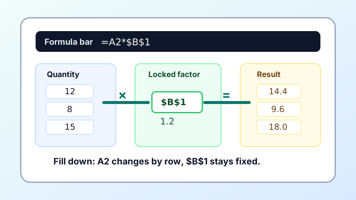
To multiply a whole column by one number, put the multiplier in one cell, lock that reference with dollar signs, and fill down. The standard formula is =A2*$B$1, where A2 changes by row and $B$1 stays fixed. Use it for tax rates, discounts, markups, and unit conversions.
Imagine column A contains quantities and cell B1 contains a conversion factor of 1.2. In C2, enter =A2*$B$1. The dollar signs tell Excel not to move the reference when you copy the formula downward. When you fill the formula down from row 2 to row 200, A2 becomes A3, A4, and so on, but $B$1 stays locked.
That one trick prevents a lot of mistakes. Without the dollar signs, Excel would slide the multiplier to B2, B3, and beyond, which is not what you want if the factor is supposed to stay fixed. Locked references are one of the most useful habits in Excel because they make formulas portable without making them fragile.
You can also use a dynamic array approach in modern Excel if you want to calculate many rows at once. For example, =A2:A10*$B$1 can spill results into multiple cells in supported versions. That is handy when you are building a quick calculation block and do not want to fill the formula manually.
If you are multiplying by a percentage, the same rule still applies. A 10% discount is simply 0.1 in Excel, so the formula might look like =A2*(1-$B$1) for a discounted total or =A2*$B$1 for a markup. The syntax changes a little, but the reference strategy stays the same.
For one-time conversions, Paste Special can also multiply a selected column by a number without leaving formulas behind. Copy the multiplier cell, select the target numbers, choose Paste Special, select Multiply, and confirm. I use formulas for live models and Paste Special only when I want to permanently transform copied values.
When should you use PRODUCT instead of the asterisk operator?
Use PRODUCT when the calculation involves a range, multiple separate arguments, or a workbook that other people will maintain. Use the asterisk operator when you only need a small, explicit calculation. In practice, PRODUCT becomes the cleaner choice as soon as the formula grows beyond a few visible references.
Here is the short version:
| Situation | Better choice | Example |
|---|---|---|
| Two cells | * | =A1*B1 |
| Three fixed cells | * or PRODUCT | =A1*B1*C1 |
| A range of values | PRODUCT | =PRODUCT(A1:A5) |
| Many inputs across a sheet | PRODUCT | =PRODUCT(A1:A10,B1:B10) |
| Readability for teammates | PRODUCT | =PRODUCT(Qty, Price, Tax) |
The operator is the simplest answer when you know exactly which cells belong in the formula. It is also the most direct because anyone reading the sheet can see the math immediately. That is why I still use * for line items, small models, and quick checks.
PRODUCT, on the other hand, earns its keep when the workbook starts to grow. It keeps long formulas shorter, which reduces visual clutter. It also makes your intent obvious: you are multiplying a set of numbers, not performing a one-off calculation. That clarity matters in spreadsheets that will be reviewed, copied, or handed off.
In Excel terms, PRODUCT is the cleaner scaling choice and * is the faster literal choice. If the formula will live for months, get copied across sheets, or be read by someone else, PRODUCT is usually easier to defend.
What causes multiplication formulas to return an error?
Multiplication formulas usually break because one input is not a real number, a copied reference moved to the wrong place, or the displayed format hides the real value. In most cases, the fix is not new math. Check the source cells, then repair data types, references, or formatting.
The most common issues are:
- Text stored as numbers. A cell may look numeric but behave like text.
- Blank cells in a chain. Depending on the formula, blanks can cause a result that is zero or misleading.
- Mixed data types. Numbers, dates, currency text, and symbols do not always play nicely together.
- Wrong reference locking. If a fixed multiplier drifts while you copy the formula, the result will be wrong even if Excel does not show an error.
- Unwanted decimal formatting. The underlying math may be fine, but the displayed result can look off if the cell format is wrong.
When I suspect a text problem, I test with VALUE, a multiply-by-1 helper, or Paste Special > Multiply. Any of those approaches can force Excel to treat the value as a number. If the issue is a bad reference, I click the formula cell and inspect the colored outlines so I can see exactly what is being multiplied.
One stray text value can break a chain of * operators, so I always check the raw source cells before I troubleshoot the formula itself. That habit saves more time than staring at the formula bar and hoping the answer appears.
Blank cells deserve a separate look. A blank in direct multiplication behaves like zero, so =A2*B2 returns zero if one side is empty. That can be correct for a missing quantity, but misleading for a missing price. If blanks mean “not ready,” wrap the formula in a simple check such as =IF(OR(A2="",B2=""),"",A2*B2).
How do you build a clean multiplication workflow?
A clean multiplication workflow starts with a simple sheet layout, one fixed calculation rule, and a formula you can copy without editing by hand. Keep inputs in their own columns, place constants in labeled cells, and choose either * or PRODUCT based on how many inputs you need.
Here is a practical example. Suppose you are pricing a list of items:
- Put quantities in column A.
- Put unit prices in column B.
- Put the result formula in column C.
- Use
=A2*B2inC2. - Fill the formula down.
That structure keeps the workbook readable and reduces copy errors. If a single rate applies to every row, store it in one dedicated cell and lock it with $. If you need to multiply a range, use PRODUCT instead of chaining many operators.
This same workflow works for tax calculations, shipping costs, commissions, and unit conversions. The exact scenario changes, but the pattern does not: separate inputs from outputs, keep one fixed reference when needed, and use the simplest formula that still reads clearly.
Before I send a workbook to anyone else, I test the first row, a middle row, and the last row. That quick three-point check catches the usual fill-down mistakes: a drifting multiplier, a blank row included by accident, or a copied formula that skipped one input column. It is faster than auditing every cell and safer than trusting the fill handle blindly.
If you need a faster mental check, remember this rule: one row, one formula; one fixed factor, one locked cell; many values, PRODUCT. That is the entire decision tree in one sentence.
What should you read next?
If multiplication is the next step in your Excel toolkit, read the matching arithmetic guides for subtraction and addition next. They reinforce the same reference habits from a different angle, especially relative references, locked references, ranges, and formulas that stay readable after you copy them through a worksheet.
Start with Excel Subtraction Formula if you want the same row-by-row pattern but with the minus operator. Then read Excel SUM Formula to compare how Excel handles addition across a range. After that, you will be ready to combine operators in more realistic models.
FAQ
The fastest multiplication answers in Excel come down to five repeatable patterns: two-cell multiplication, long chains, fixed multipliers, text-value cleanup, and model readability. Each answer below includes a number because formula decisions are easier when you know the scale, limit, or row pattern you are choosing around.
What is the fastest way to multiply two cells in Excel?
The fastest way is still =A1*B1, because it uses 1 operator and only 2 references. For a quick check or a single line item, that is usually faster than opening the function picker or typing a longer function name.
Can PRODUCT replace a long chain of asterisks?
Yes. PRODUCT can replace a chain that grows to 5, 10, or even 20 inputs, and it can take up to 255 arguments. That makes it much easier to read than =A1*B1*C1*D1....
How do I multiply every row by the same value?
Put the fixed value in 1 cell, lock it with $, and fill down. A formula like =A2*$B$1 keeps the multiplier constant while Excel adjusts the row reference for each new line.
Why do text values break multiplication?
1 text value can break a * chain because Excel expects numbers on both sides of the operator. Convert the text first, and then the same formula often works without any other change.
Is PRODUCT better for large models?
It often is, especially when you are multiplying more than 3 or 4 inputs. Microsoft lists 255 as the function-argument limit, so PRODUCT gives you plenty of room while keeping shared workbook formulas easier to audit.
