
Excel’s #SPILL! error means a dynamic array formula produced more than one result but cannot place every result in the worksheet. The fastest fix is to select the error, inspect the outlined spill range, and clear or move anything occupying it. If nothing visible blocks the range, check tables, merged cells, worksheet edges, and changing array sizes.
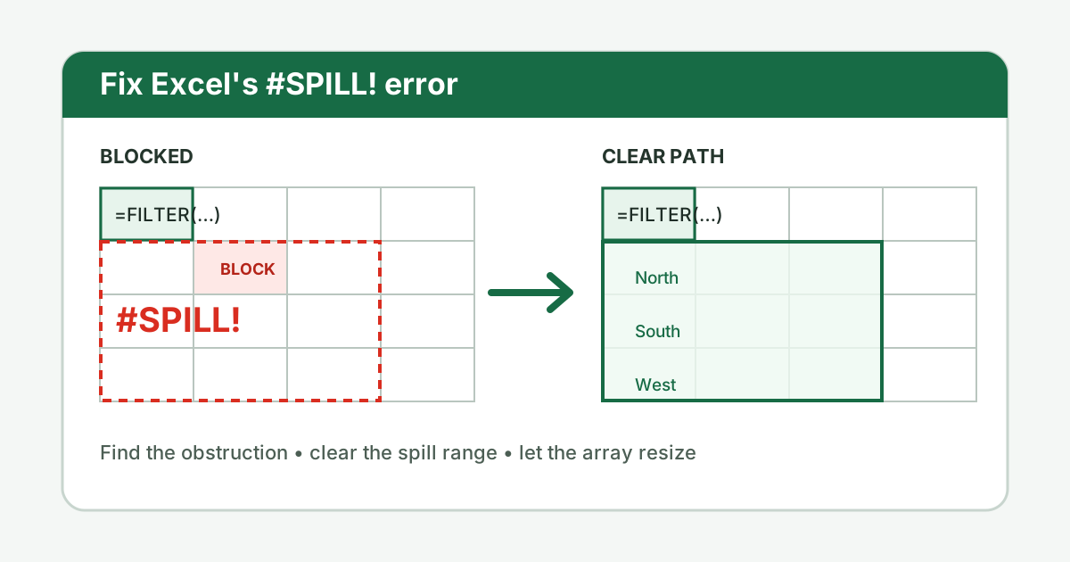
Microsoft fact: Dynamic array formulas automatically return results into neighboring cells, and only the top-left cell is editable. Microsoft calls that output area the spill range in its guide to dynamic array formulas and spilled array behavior.
Quick fix: select the #SPILL! cell, click its warning icon, and read the reason. If Excel reports that the spill range is not blank, choose Select Obstructing Cells, remove or relocate the obstruction, and recalculate. Do not delete source data until you have confirmed that the selected cell really belongs in the output area.
What does #SPILL! mean in Excel?
The #SPILL! error means Excel knows the array of answers a formula should return, but the intended output area is unavailable or indeterminate. The formula itself may be valid. Excel displays the error in the top-left formula cell because it cannot populate the full spill range safely.
Modern functions such as FILTER, SORT, SORTBY, UNIQUE, SEQUENCE, RANDARRAY, and some uses of XLOOKUP can return several values from one formula. Excel places those values in adjacent cells automatically. This is a dynamic array spill, and the occupied rectangle is the spill range.
For example, this formula can return every matching row from A2:C100:
=FILTER(A2:C100,C2:C100="Open","No open rows")If the result contains nine rows and three columns, Excel needs a clear 9-by-3 area beginning at the formula cell. One value, a formula, or a merged cell anywhere in that rectangle can prevent the whole result from appearing.
The error therefore differs from #N/A or #VALUE!. Those errors usually describe a lookup or calculation problem. #SPILL! describes a placement problem, although a few causes—such as an array whose size keeps changing—come from formula design rather than a visible obstruction.
How do you fix a blocked spill range?
Fix a blocked spill range by selecting the #SPILL! cell, identifying the outlined destination, and clearing only the cells that should be empty. Excel’s warning menu may offer Select Obstructing Cells, which is safer than scanning a large range or deleting a whole worksheet area blindly.
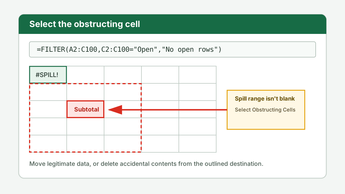
Use this sequence:
- Select the cell displaying
#SPILL!. - Look for the dashed border showing the intended spill range.
- Click the warning icon beside the selected cell.
- Choose Select Obstructing Cells if Excel offers it.
- Inspect the selected cell’s value or formula.
- Delete it only if it is accidental; otherwise move the dynamic array formula to a clear location.
A cell can look empty while still containing a formula that returns "", an apostrophe, or a space. Press Delete to clear unwanted contents rather than using the spacebar. If existing data is legitimate, preserve it and place the formula where its output has enough room.
Microsoft’s official #SPILL! troubleshooting page documents Spill range isn’t blank as a primary cause and describes the obstructing-cell command. That diagnostic is the best first step because Excel knows the exact rectangle the formula tried to use.
Why do merged cells cause a spill error?
Merged cells cause #SPILL! because a dynamic array needs individual worksheet cells for each result, while a merged region replaces several grid positions with one display area. Unmerge any cells inside the proposed spill range, or move the formula and output to an unmerged reporting area.
To repair the layout, select the merged cell, then use Home > Merge & Center > Unmerge Cells. Keep the cells unmerged and use alignment or formatting for presentation. If the merge belongs to a title or dashboard section, moving the formula is usually cleaner than redesigning that section.
The dashed spill border helps reveal a partial overlap. A merge several rows below the formula can block the entire result even when the first few destination cells are clear. Excel does not return a truncated answer because that would silently omit valid array results.
Merged cells are especially easy to miss in templates. Check row heights, centered headings, and copied report blocks if the warning menu says the range contains merged cells but the blockage is not obvious.
Can spilled array formulas work inside Excel tables?
Spilled array formulas cannot spill from cells inside an Excel table. Move the formula into the ordinary worksheet grid outside the table. The source data can remain in a table, and the external formula can use structured references, but its expanding results need a non-table destination.
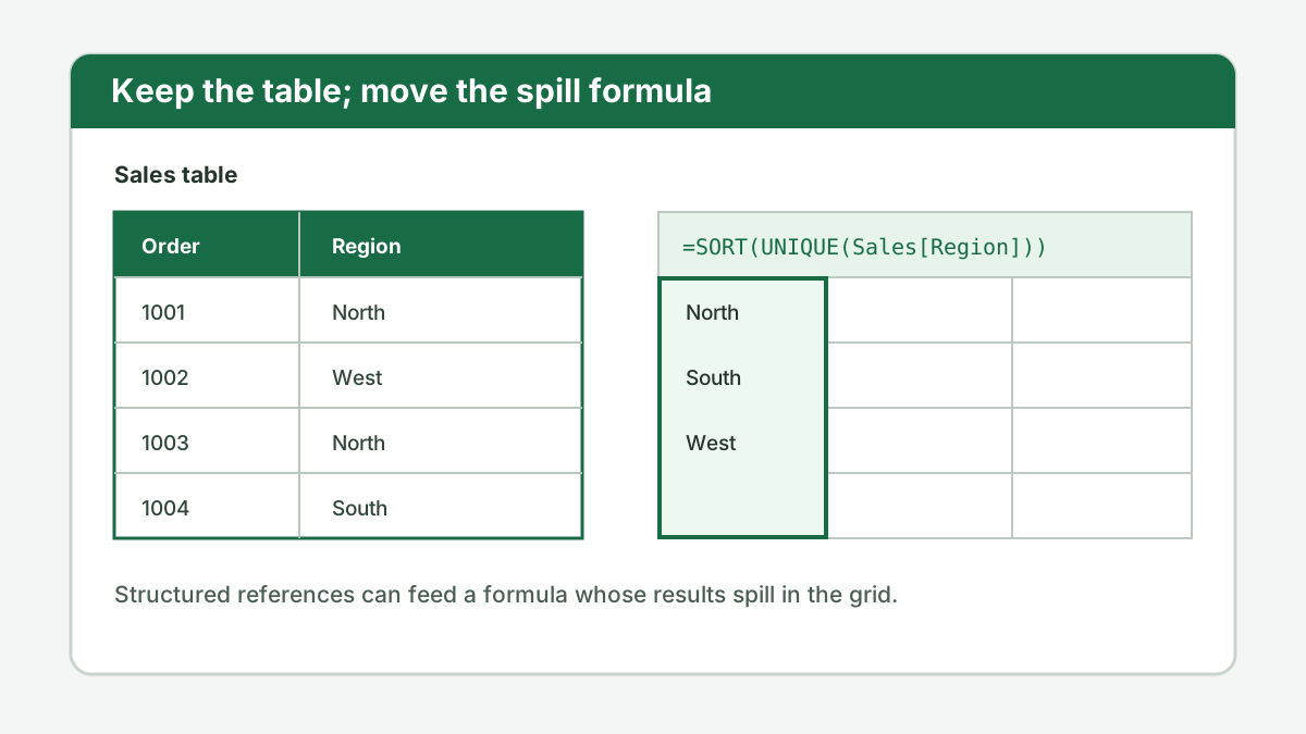
Suppose a table named Sales contains a Region column. Place this formula in a clear cell outside the table:
=SORT(UNIQUE(Sales[Region]))The formula can still react when rows are added to Sales, while its spill range expands independently in the grid. Microsoft explicitly notes that spilled array formulas are not supported inside Excel tables, although structured references are appropriate inputs.
Do not confuse a formula outside a table with source data outside a table. Tables remain useful because their structured references resize as records are added. Only the top-left dynamic array formula and its returned spill cells must sit outside the table boundary.
If you are building a distinct list from table data, Excel UNIQUE Ignore Blanks shows how to combine UNIQUE and FILTER. Leave enough empty grid space below and to the right of that formula.
How do worksheet edges and full-column references create #SPILL!?
Worksheet edges create #SPILL! when an array would extend beyond Excel’s available rows or columns. Full-column references can trigger the same problem if the formula starts below row 1, because returning an entire column from that position would require more rows than remain in the sheet.
Microsoft documents this example entered in E2, where the whole-column lookup value makes Excel return 1,048,576 results and run past the bottom of the grid:
=VLOOKUP(A:A,A:C,2,FALSE)Prefer a bounded lookup range when you want several results:
=VLOOKUP(A2:A5000,A:C,2,FALSE)If you want only the value from the formula’s row, use explicit implicit intersection instead:
=VLOOKUP(@A:A,A:C,2,FALSE)The @ operator reduces A:A to the value on the same row, so this version returns one result rather than a dynamic array. Microsoft shows both repairs on its official #SPILL! troubleshooting page. Better still, store multi-row source data in a table and use a structured reference that grows without demanding every worksheet row.
Also check horizontal formulas near column XFD and vertical formulas near row 1,048,576. Move the top-left formula upward or leftward, reduce the returned array, or place the output on a new sheet with sufficient space.
Why does Excel say the spill range is unknown?
Excel reports an unknown or indeterminate spill size when a formula’s array dimensions keep changing between calculation passes. Stabilize the size by removing volatile size logic, setting a fixed limit, or redesigning the formula so Excel can determine one final output rectangle before placing results.
A classic example combines SEQUENCE with a volatile result:
=SEQUENCE(RANDBETWEEN(1,1000))RANDBETWEEN may produce a different row count each time Excel recalculates the formula. Excel makes additional calculation passes to resolve the array. If the dimensions do not stabilize, it returns #SPILL! rather than writing a moving target into the grid.
Use a fixed size when possible:
=SEQUENCE(100)If the size must be user controlled, put the requested count in a validated input cell and reference that cell:
=SEQUENCE(MIN(MAX(B1,1),1000))That version caps the output between 1 and 1,000 rows. It is more predictable, easier to audit, and less likely to make downstream formulas change shape unexpectedly.
What is the spill range operator in Excel?
The spill range operator is the # appended to the top-left cell reference of a dynamic array result. If a formula in E2 spills through E10, E2# refers to that entire current range and automatically adjusts when the number of returned rows changes.
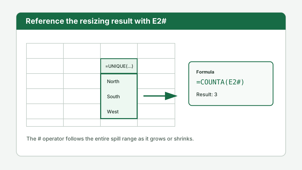
For example:
=COUNTA(E2#)This counts the current values returned by the dynamic array that begins in E2. You do not need to guess its last row or maintain a fixed reference such as E2:E100.
You can also pass a spill range into another function:
=SORT(E2#)Only the top-left cell contains the dynamic array formula. Other cells in the spill range are results and cannot be edited individually. To change the calculation, edit the top-left formula; to remove the result, delete that formula.
This behavior is useful with lookups. An XLOOKUP can return multiple adjacent columns when its return array includes them, and another formula can refer to the resulting spill with #. See the site’s Excel XLOOKUP guide for lookup syntax and matching options.
How do you prevent future #SPILL! errors?
Prevent future #SPILL! errors by reserving clear output areas, keeping dynamic formulas outside tables, avoiding merged destination cells, and using bounded or structured source references. Build downstream calculations with the # operator so they follow the spill range instead of imposing fixed endpoints that become outdated.
These habits make dynamic-array workbooks more resilient:
- Put source records in tables, but put spilling formulas in the grid.
- Leave buffer space below and to the right of each dynamic result.
- Do not type manual notes or subtotals inside a potential spill area.
- Avoid merged cells in calculation zones.
- Prefer table columns or realistic bounded ranges over entire columns.
- Use the formula’s
[if_empty]argument when available; it handles no matches, not blocked outputs. - Reference the completed output as
E2#instead of guessing its last cell. - Label the top-left formula so collaborators know the neighboring cells are reserved.
Remember that blank results and blank destination cells are different. FILTER can return a fallback such as "No matches" when no rows qualify, but [if_empty] cannot repair an occupied spill range. Clear the obstruction or move the formula.
When sharing a workbook with users on older Excel versions, verify compatibility too. Dynamic arrays are a modern Excel feature; older versions may show implicit-intersection behavior or compatibility syntax instead of an editable spill range.
What should you check when #SPILL! keeps returning?
When #SPILL! keeps returning, diagnose the reason shown in Excel’s error menu rather than repeating the same clear-and-recalculate step. Persistent cases usually involve hidden contents, merged cells, table placement, worksheet boundaries, full-column arrays, or formulas whose output dimensions change during recalculation.
Work through this checklist:
- Confirm you selected the top-left formula cell, not a neighboring result.
- Use Select Obstructing Cells and inspect formulas as well as displayed values.
- Clear spaces, apostrophes, and formulas that display empty text.
- Unmerge every cell touched by the dashed border.
- Move the formula outside any Excel table.
- Replace full-column inputs with table references or bounded ranges.
- Move the formula away from the bottom or right worksheet edge.
- Replace volatile array-size expressions with stable, capped inputs.
- Check whether another spilled formula overlaps the same destination.
Calculation mode is rarely the root cause, but press F9 after fixing the layout if the workbook uses manual calculation. If the error returns only as source data grows, the reserved output area is too small or another report element sits too close to it.
Summary
To fix an Excel #SPILL! error, start at the top-left formula, read the warning reason, and inspect the outlined spill range. Clear or move true obstructions, unmerge destination cells, keep dynamic formulas outside tables, bound oversized references, and stabilize formulas whose array dimensions change between calculation passes.
The essential distinction is simple: a spill error usually means Excel cannot place a valid multi-cell result, not that every part of the formula is wrong. Protect a clear output area and let one formula control it. Then use a reference such as E2# whenever another calculation needs the complete, resizing result.
FAQ
These common #SPILL! questions cover the meaning of the error, the fastest obstruction check, table restrictions, the spilled-range operator, and persistent layout or formula causes. Use the error menu first because its reason narrows the repair before you change source data or rebuild a formula that may already be correct.
What does #SPILL! mean in Excel?
#SPILL! means a dynamic array formula calculated multiple results but cannot place them all in the worksheet grid. Select the formula cell and use Excel’s dashed spill-range outline or error menu to identify what is blocking or constraining the output.
How do I find the cell blocking a spill range?
Select the #SPILL! cell, open its error menu, and choose Select Obstructing Cells when that option appears. Excel jumps to the blocking cell. You can also inspect every cell inside the dashed spill-range border for values, spaces, merged cells, or other formulas.
Can a dynamic array formula spill inside an Excel table?
No. Spilled array formulas are not supported inside Excel tables. Put the formula in the worksheet grid outside the table, while still using structured references to the table as the source. The results can then resize when table data changes.
What does the # symbol mean in an Excel formula reference?
A # after the top-left cell address is the spilled-range operator. For example, E2# refers to the complete dynamic spill range that begins in E2. The reference expands or contracts automatically when the source formula returns a different number of results.
Why does #SPILL! return after I clear the visible cells?
The formula may still be inside a table, overlap merged cells, reference an entire column, reach the worksheet edge, or use a volatile expression whose result size keeps changing. Open the error menu for the specific reason, then correct that layout or formula condition.
