
Use =UNIQUE(A2:A100) to extract unique values from a column in current Excel. Enter the formula once in an empty cell, press Enter, and the results spill downward automatically. Add FILTER when you need criteria or want to exclude blanks, and use the third argument when you need values that occur exactly once.
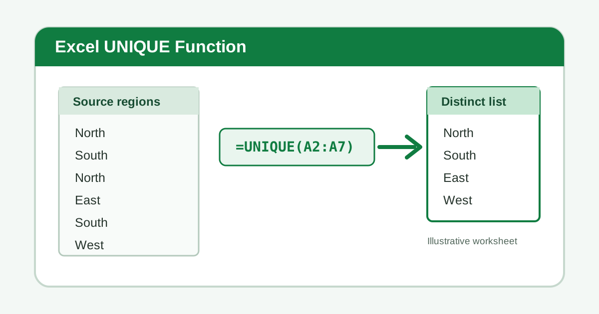
Sourced Excel fact: Microsoft documents three UNIQUE arguments—one required
arrayargument and two optional arguments,by_colandexactly_once. The result is a dynamic array that spills into neighboring cells automatically.Source: Microsoft Support — UNIQUE function (accessed July 24, 2026).
| Goal | Formula |
|---|---|
| Extract a distinct list | =UNIQUE(A2:A100) |
| Sort the distinct list | =SORT(UNIQUE(A2:A100)) |
| Ignore blank cells | =UNIQUE(FILTER(A2:A100,A2:A100<>"")) |
| Apply one criterion | =UNIQUE(FILTER(A2:A100,B2:B100="West")) |
| Return values appearing once | =UNIQUE(A2:A100,,TRUE) |
| Extract distinct rows | =UNIQUE(A2:C100) |
Key takeaways
UNIQUEcreates a live distinct list without changing the source data.- A multi-column array returns distinct row combinations, not separate lists per column.
FILTERshould run insideUNIQUEwhen you need conditions or blank removal.- The optional
exactly_onceargument finds true single-occurrence records. - A clear spill range is required; the formula itself belongs outside an Excel Table.
How Do You Use the UNIQUE Function in Excel?
Enter =UNIQUE(range) in the first cell where you want the distinct list to begin, then press Enter. Excel evaluates the source, keeps one instance of each different value or row, and spills the results into adjacent cells. The source remains unchanged, and the output updates whenever its referenced data changes.
Suppose A2:A9 contains North, South, North, East, South, West, East, and North. In C2, enter:
=UNIQUE(A2:A9)Cells C2:C5 display North, South, East, and West. You do not copy the formula down. Only C2 contains the formula; the other cells are spill results controlled by that anchor cell.
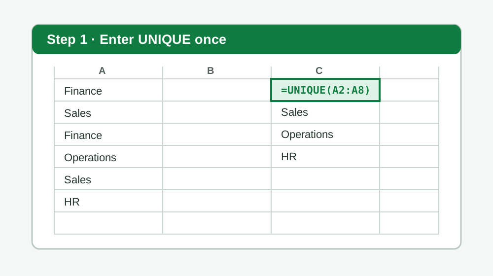
Choose an output cell with empty space beneath it. Excel shows a blue outline around the complete spill range when you select the formula cell. If the source is an Excel Table, structured references make the result especially useful:
=UNIQUE(Sales[Region])When rows are added to Sales, the distinct region list expands or contracts automatically. Put the formula outside the Table, because spilled array formulas cannot live inside Table columns.
For a polished alphabetical list, wrap the formula in SORT:
=SORT(UNIQUE(Sales[Region]))This approach is ideal for validation lists, report labels, dashboard selectors, and quick data-quality checks. It creates a formula-driven output rather than deleting or overwriting any record.
What Is the UNIQUE Function Syntax?
The syntax is =UNIQUE(array,[by_col],[exactly_once]). array is the source range. Leave by_col omitted or FALSE to compare rows; use TRUE to compare columns. Leave exactly_once omitted or FALSE for one copy of every distinct item; use TRUE to return only items appearing one time.
Here is what each argument controls:
| Argument | Required? | Meaning |
|---|---|---|
array | Yes | Range or array containing the values or records |
by_col | No | FALSE compares rows; TRUE compares columns |
exactly_once | No | FALSE returns distinct items; TRUE returns single-occurrence items |
The basic formula below compares entries down a column:
=UNIQUE(A2:A100)For a horizontal source in B2:G4, setting by_col to TRUE compares complete columns:
=UNIQUE(B2:G4,TRUE)That is different from turning a vertical result horizontal. If you only want the basic list to display across columns, use:
=TRANSPOSE(UNIQUE(A2:A100))The third argument is often misunderstood. The default formula returns each distinct value once, even when that value appeared many times. exactly_once set to TRUE excludes every repeated value:
=UNIQUE(A2:A100,,TRUE)If Ana appears three times, Ben twice, and Chen once, ordinary UNIQUE returns Ana, Ben, and Chen. The exactly-once formula returns only Chen. That makes it useful for spotting unmatched IDs, one-time customers, or records that failed to repeat when repetition was expected.
How Do You Extract Unique Values and a Distinct List?
To extract unique values from one field, reference that column; to extract distinct records, reference every column that defines the record. =UNIQUE(A2:A100) compares individual cells, while =UNIQUE(A2:C100) compares whole rows and retains one copy of each different three-column combination in the resulting spill array.
Imagine columns A through C contain Customer, Region, and Product. Two rows count as duplicates only if all three values match. A repeated customer with a different product remains because the complete row is distinct:
=UNIQUE(A2:C100)This distinction matters when people say “unique list.” They may mean unique customer names, unique customer-region pairs, or records that occur exactly once. Define the unit first, then select the matching array.
To reorder the output by customer and then region, add SORT:
=SORT(UNIQUE(A2:C100),{1,2},{1,1})For unique values from nonadjacent fields, combine columns with CHOOSE:
=UNIQUE(CHOOSE({1,2},A2:A100,C2:C100))That formula builds a temporary two-column array from columns A and C, then returns distinct row combinations. Keep ranges the same height; mismatched array dimensions cause errors or misleading output.
If your goal is a number rather than the extracted values, see how to count unique values in Excel. A common count is:
=ROWS(UNIQUE(FILTER(A2:A100,A2:A100<>"")))ROWS is reliable for a vertical list and makes the relationship clear: first build the distinct list, then count its rows. Inspecting the spill list before counting is a useful audit step when the total looks unexpected.
How Do You Combine UNIQUE with FILTER?
Place FILTER inside UNIQUE so Excel applies the conditions first and deduplicates only the matching rows. For example, =UNIQUE(FILTER(A2:A100,B2:B100="West")) keeps values from column A where column B equals West, then returns one copy of each matching value as a dynamic distinct list.
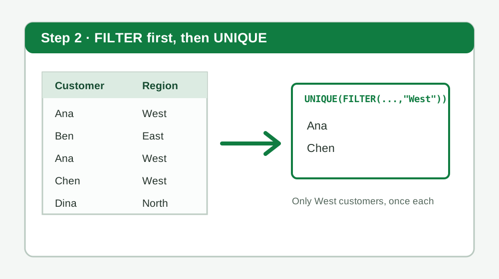
With customer names in column A and regions in column B, use:
=UNIQUE(FILTER(A2:A100,B2:B100="West","No matches"))The "No matches" argument belongs to FILTER and prevents a #CALC! error when no row meets the condition. It becomes part of the array passed to UNIQUE, so choose a message that is clear to the report reader.
For two AND conditions, multiply the Boolean tests. This returns distinct products from column A for West rows with sales of at least 1,000:
=UNIQUE(FILTER(A2:A100,(B2:B100="West")*(C2:C100>=1000),"No matches"))For OR logic, add the tests. This returns distinct products sold in either West or East:
=UNIQUE(FILTER(A2:A100,(B2:B100="West")+(B2:B100="East"),"No matches"))You can make the criterion interactive by replacing "West" with a cell:
=SORT(UNIQUE(FILTER(A2:A100,B2:B100=E2,"No matches")))When the user changes E2, the sorted distinct list refreshes. This pattern works well for dashboard helper ranges and dependent drop-down sources. Avoid whole-column references inside several nested dynamic-array functions when a bounded range or Table reference will do; smaller inputs are easier to audit and usually calculate more efficiently.
How Do You Make UNIQUE Ignore Blanks?
Filter blank cells out before UNIQUE sees them: =UNIQUE(FILTER(A2:A100,A2:A100<>"")). The comparison creates TRUE for populated cells and FALSE for empty cells; FILTER keeps the populated values, then UNIQUE reduces them to a distinct list. This prevents ordinary UNIQUE from including a result for source blanks, which Excel can display as 0.
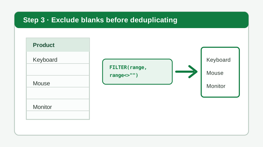
Use a fallback when the source could be entirely empty:
=UNIQUE(FILTER(A2:A100,A2:A100<>"","No values"))Cells that look blank may contain formulas returning "", spaces, or other invisible characters. The <>"" test excludes true empties and zero-length formula results, but a cell containing one space is still text. If imported data contains stray spaces, clean it before deduplication:
=LET(clean,TRIM(A2:A100),UNIQUE(FILTER(clean,clean<>"","No values")))TRIM removes standard extra spaces, LET names the cleaned array, and the remaining functions filter and deduplicate it. For nonbreaking spaces copied from web pages, use SUBSTITUTE with CHAR(160) before TRIM:
=LET(clean,TRIM(SUBSTITUTE(A2:A100,CHAR(160)," ")),UNIQUE(FILTER(clean,clean<>"","No values")))Cleaning changes the values used for comparison, so confirm that whitespace is not meaningful in codes or identifiers. For a deeper treatment of empty-string formulas, multiple columns, and compatibility options, read Excel UNIQUE: ignore blanks.
How Do You Return Values That Occur Exactly Once?
Set the third argument to TRUE: =UNIQUE(A2:A100,,TRUE). This does not merely remove duplicates. It discards every value that appears two or more times and returns only single-occurrence values. Leave the second argument blank because you are comparing rows, then activate exactly_once with the final TRUE value.
This is useful for reconciliation. If two exports should contain matching invoice IDs, stack the IDs into one array and return those appearing only once:
=LET(ids,VSTACK(A2:A100,D2:D100),UNIQUE(FILTER(ids,ids<>""),,TRUE))Any ID present in both lists normally appears twice and is excluded. IDs present in just one list remain for investigation. If one export can contain internal duplicates, this quick pattern may hide an issue; summarize or validate each source first when duplicate IDs are possible.
For complete records, provide multiple columns:
=UNIQUE(A2:C100,,TRUE)Excel returns rows whose entire A:C combination occurs exactly once. A duplicated customer name does not disqualify a row if its other fields differ. That is why selecting the correct array is as important as setting the argument.
To highlight one-time values beside the source rather than extract them, COUNTIF is often more appropriate:
=COUNTIF($A$2:$A$100,A2)=1Fill that helper formula down and filter TRUE. Use UNIQUE(...,,TRUE) when you need a compact spill list; use a helper when you need to preserve row context or review every source record in place.
Why Is the UNIQUE Function Not Working?
First check for blocked spill cells, merged cells, Table placement, unsupported Excel versions, and closed-workbook links. A #SPILL! error means Excel cannot place the result; #NAME? usually means the function is unavailable. #REF! can appear when a dynamic-array formula references a closed external workbook, according to Microsoft.
Click the error cell and inspect Excel’s warning menu. For #SPILL!, Excel normally outlines the intended result area. Clear values, formulas, or merged cells inside that outline. Remember that a cell containing an invisible formula is not empty.
Other common fixes include:
- Move the formula outside an Excel Table.
- Replace full-column arrays if the spill would run beyond row 1,048,576.
- Make all
FILTERranges the same height and width. - Open linked source workbooks before recalculation.
- Confirm the workbook is being opened in a version that supports
UNIQUE.
Microsoft lists UNIQUE for Microsoft 365, Excel 2021, Excel 2024, Excel for the web, and current mobile editions. Older perpetual versions such as Excel 2019 do not support it. For shared files, ask collaborators which version they use before building a critical workflow around dynamic arrays.
If the output contains apparent duplicates, inspect data types and hidden characters. The number 1001 and text "1001" can behave differently, while trailing or nonbreaking spaces make labels visually similar but technically distinct. Test suspicious cells with ISTEXT, ISNUMBER, LEN, or EXACT, then normalize the source deliberately.
Frequently Asked Questions
These quick answers cover the most common UNIQUE function decisions: the basic distinct-list formula, blank removal, criteria, spill errors, and single-occurrence values. Each formula assumes a current Excel version with dynamic arrays and an empty output area. Use bounded ranges or Table references when possible so formulas remain readable and responsive.
What is the Excel formula for unique values?
Use =UNIQUE(A2:A100) to return one copy of every distinct value in the range. Enter the formula in an empty cell with clear space below it, and Excel spills the resulting list into as many cells as needed.
How do I use UNIQUE without blanks?
Filter the source before deduplicating it: =UNIQUE(FILTER(A2:A100,A2:A100<>"")). FILTER removes empty cells, then UNIQUE returns the distinct remaining values. If the source can contain no populated cells, use FILTER’s optional if_empty argument to provide a fallback.
Can UNIQUE return values based on criteria?
Yes. Put FILTER inside UNIQUE, such as =UNIQUE(FILTER(A2:A100,B2:B100="West","None")). FILTER keeps only rows where column B is West, and UNIQUE reduces the matching values from column A to a distinct list.
Why does my UNIQUE formula show a SPILL error?
A SPILL error usually means something occupies the intended output area, the formula sits inside an Excel Table, merged cells block the range, or the output would cross the worksheet edge. Select the warning indicator, clear the highlighted obstruction, and keep the formula outside tables.
What does exactly_once do in UNIQUE?
Set UNIQUE’s third argument to TRUE to return only values or rows that occur exactly once, for example =UNIQUE(A2:A100,,TRUE). The default FALSE behavior returns one copy of every distinct item, including items that appeared multiple times in the source.
What Should You Remember About Excel UNIQUE?
Use UNIQUE when you need a live, non-destructive distinct list. Start with =UNIQUE(range), add SORT for presentation, put FILTER inside it for conditions or blank removal, and use exactly_once only for single-occurrence records. Keep the spill area clear and verify the selected columns match your definition of a record.
The best formula is usually the simplest one that answers the actual question. Decide whether “unique” means one copy of every distinct item or only items occurring once; decide whether blanks count; then decide whether criteria should limit the source. Those three choices determine the correct formula more reliably than trial and error.
