
To add Change Case to the Excel Ribbon, create three small VBA macros - uppercase, lowercase, and proper case - then add each macro as a button in a custom Ribbon group. If your goal is only to rename Ribbon tab labels, skip the macro section and use File > Options > Customize Ribbon > Rename.
These are two different Excel customizations. A Change Case button changes selected worksheet text; renaming a Ribbon tab changes labels such as Data or Review in the interface.
| Goal | Best Excel feature | What changes |
|---|---|---|
| Convert selected cells to UPPERCASE, lowercase, or Proper Case | VBA macro assigned to Ribbon buttons | Cell text in the worksheet |
| Add buttons to the Home tab | Customize Ribbon | Ribbon commands available to you |
| Rename tabs such as Data or Review | Customize Ribbon > Rename | Ribbon tab labels only |
Add Change Case Macro Buttons to the Excel Ribbon
Excel does not include Word’s built-in Change Case command. The closest native formula options are UPPER, LOWER, and PROPER, but those return results in helper cells instead of changing the selected cells in place.
A Ribbon macro is useful when you regularly clean imported names, product labels, addresses, or report headings. I prefer three separate buttons because they avoid the clunky pop-up prompt and make the Ribbon behavior predictable.
Enable the Developer Tab
First, show the Developer tab so you can add the macro code.
- Click File > Options > Customize Ribbon.
- In the right-hand list, check Developer.
- Click OK.
You only need to do this once. After the Developer tab is visible, it stays on the Ribbon unless you hide it again.
Add the VBA Macros
Open Developer > Visual Basic, then choose Insert > Module. Paste this code into the module:
Option Explicit

Private Sub ApplyCaseToSelection(ByVal caseMode As String)
    Dim cell As Range

    If TypeName(Selection) <> "Range" Then Exit Sub

    For Each cell In Selection.Cells
        If Not cell.HasFormula Then
            If Len(cell.Value2) > 0 Then
                Select Case caseMode
                    Case "upper"
                        cell.Value = UCase$(CStr(cell.Value))
                    Case "lower"
                        cell.Value = LCase$(CStr(cell.Value))
                    Case "proper"
                        cell.Value = StrConv(CStr(cell.Value), vbProperCase)
                End Select
            End If
        End If
    Next cell
End Sub

Sub ChangeCaseUpper()
    ApplyCaseToSelection "upper"
End Sub

Sub ChangeCaseLower()
    ApplyCaseToSelection "lower"
End Sub

Sub ChangeCaseProper()
    ApplyCaseToSelection "proper"
End Sub
This version skips formula cells so it does not overwrite calculations. It changes only non-empty selected cells, which is safer than running a broad macro across an entire worksheet.
Save the workbook as a macro-enabled file (.xlsm) before you close Excel. Standard .xlsx files cannot store VBA macros.
Add the Macros to a Custom Ribbon Group
Now add the three macros to the Ribbon.
- Click File > Options > Customize Ribbon.
- Select the tab where you want the buttons, usually Home.
- Click New Group, then rename it to Text Tools or Change Case.
- In Choose commands from, select Macros.
- Add
ChangeCaseUpper,ChangeCaseLower, andChangeCaseProperto the new group. - Select each macro, click Rename, and choose a short display name such as UPPER, lower, and Proper.
- Click OK.
The commands now appear in your custom Ribbon group. Select a few text cells and click the button you want.
Test the Buttons Safely
Before using the macros on real data, test them on copied sample values:
| Sample value | UPPER button | lower button | Proper button |
|---|---|---|---|
| north region | NORTH REGION | north region | North Region |
| JANE SMITH | JANE SMITH | jane smith | Jane Smith |
| product id a17 | PRODUCT ID A17 | product id a17 | Product Id A17 |
Proper case is helpful for names and labels, but it is not perfect for every acronym. For example, product id a17 becomes Product Id A17, so review technical labels after conversion.
Can You Make One Dropdown Instead?
Excel’s built-in Customize Ribbon dialog can add macro buttons, but it cannot create a true custom dropdown menu. If you want one Change Case dropdown with three choices inside it, you need Ribbon XML, an add-in, or a tool such as Office RibbonX Editor.
For most users, three macro buttons are faster to build and easier to maintain. They also avoid the old pop-up prompt pattern where the macro asks you to type 1, 2, or 3 every time you run it.
Formula Alternative Without Macros
If you cannot use macros, use helper formulas instead. Put the original text in column A, then use one of these formulas in column B:
=UPPER(A2)
=LOWER(A2)
=PROPER(A2)
Fill the formula down, copy the results, and use Paste Special > Values if you want to replace the original text. This method is slower for repeated cleanup work, but it is safer in locked-down workbooks because it does not require macro permissions.
Use formulas when the workbook must stay as .xlsx, when you are sharing the file with people who cannot enable macros, or when you want the converted text to update automatically if the source cell changes. Use the Ribbon macro buttons when you want a one-click cleanup command for selected cells.
Rename Ribbon Tab Labels in Excel
Renaming a Ribbon tab is a separate task. It does not change worksheet text, and it does not add a Change Case command. It only changes the label that appears on the Ribbon.
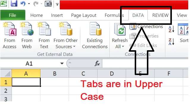
This is useful if you want tab names to match your team’s terminology. For example, you can rename Data to DATA, Review to REVIEW, or a custom tab to Monthly Close.
Open Customize Ribbon
Go to File > Options > Customize Ribbon.
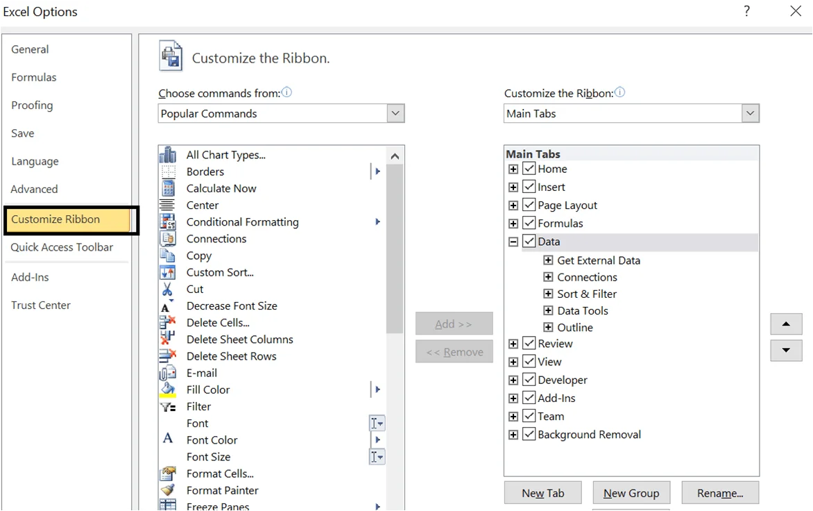
The right-hand list shows the main tabs currently available on your Ribbon. Checked tabs are visible. Unchecked tabs are hidden.
For a broader walkthrough of Ribbon settings, see our guide to customizing the Excel Ribbon.
Rename the Tab
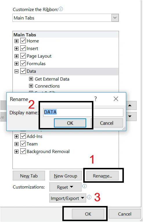
- Select the tab you want to rename.
- Click Rename.
- Type the new display name.
- Click OK in the Rename dialog.
- Click OK again to close Excel Options.
The tab label updates immediately. If you renamed Data to DATA, the Ribbon now shows the uppercase label.
You can repeat the same steps for other built-in tabs or for custom tabs that you created yourself. If you want to reverse the change later, return to the same dialog and rename the tab again.
Common Problems
My Macros Do Not Appear in the Commands List
Confirm the workbook is saved as .xlsm and that the macros are in a standard module, not inside a worksheet object. Then reopen File > Options > Customize Ribbon and choose Macros from the command list.
Excel Blocks the Macro
Excel may block macros in files downloaded from the internet. Save the workbook in a trusted location or unblock the file through Windows file properties if you trust the source.
The Macro Changes Too Much Text
The macro runs on the current selection. Select only the cells you want to change before clicking the Ribbon button. If you accidentally change too much, press Ctrl+Z immediately.
Proper Case Changes Acronyms
StrConv(..., vbProperCase) treats each word mechanically. It does not know that ID, URL, SKU, or USA should stay uppercase. Use the proper-case macro for names and ordinary labels, then manually review acronyms.
FAQ
Does Excel have a built-in Change Case button?
No. Excel has formulas such as UPPER, LOWER, and PROPER, but it does not have Word’s one-click Change Case command. A macro button is the simplest way to add that behavior to the Ribbon.
Can I add Change Case to Excel for the web?
No, not with VBA. Excel for the web does not run VBA macros. Use desktop Excel for the Ribbon macro approach, or use worksheet formulas if you need a web-compatible method.
Is renaming a Ribbon tab the same as changing case in cells?
No. Renaming a Ribbon tab only changes the interface label. It will not convert worksheet text. To change selected cell text, use the VBA macro buttons above.
