
Freezing a column in Excel keeps the left side of your worksheet visible while the rest of the sheet scrolls horizontally. That makes wide tables easier to read because the labels, IDs, or reference fields you rely on stay pinned in view. If you only need the top row instead, see how to freeze a row in Excel.
This guide shows the exact menu path, the keyboard shortcut, and the rules for freezing more than one column or combining frozen columns with frozen rows. It also includes a quick stat block, because the feature matters most once a worksheet grows from a handful of fields into a genuinely large working file.
Stat block
On 2026-07-02, the content plan recorded the target keyword how to freeze a column in excel at 18,100 monthly searches with KD 2. Microsoft support also documents that an Excel worksheet can hold 1,048,576 rows and 16,384 columns, which is why Freeze Panes becomes a readability tool long before the sheet runs out of space.
Source: content-strategy/blog-keyword-plan-2026-07.md · Microsoft Excel support
What freezing a column in Excel actually does
Freezing a column keeps key labels visible while you scroll left and right. It is a view change, not a data change: the cells, formulas, filters, and file contents all stay the same. That is why a simple freeze can make wide sheets easier to read without affecting how the workbook works.
That separation matters. Freezing is a view setting, not a data change. If you send the workbook to someone else, the freeze travels with the file, but it does not alter what is in the cells. The same sheet can still be filtered, sorted, edited, printed, and recalculated normally. The only thing that changes is the on-screen anchor point.
There are three related commands worth remembering:
| Command | What it freezes | Best use |
|---|---|---|
| Freeze First Column | Column A only | Simple lists, lookup sheets, and reports with one key identifier |
| Freeze Panes | Everything above and left of the selected cell | Multiple columns, multiple rows, or both together |
| Unfreeze Panes | Removes the current freeze | Changing the frozen area or starting over |
If your worksheet is only wide because of one important identifier column and a few data columns, freezing the first column is often enough. If the sheet is wide because the top row and left-side labels both matter, use Freeze Panes instead of trying to force the simpler command to do a bigger job.
How to freeze the first column in Excel
The fastest way to freeze a single column is to use the built-in Freeze First Column command. That locks column A in place, which is exactly what you want for a lot of common reports: customer lists, invoice exports, transaction ledgers, and any table where the first field is the field you read first.
Here is the basic path:
- Open the worksheet.
- Go to the View tab.
- Choose Freeze Panes.
- Click Freeze First Column.
If you prefer shortcuts on Windows, the sequence is Alt+W+F+C. That is useful when you are doing the same action over and over, because it avoids the menu hunt and gives you a consistent rhythm.
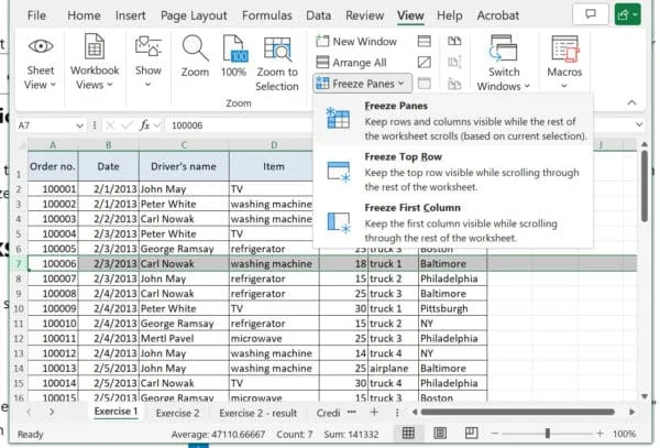 Excel freeze panes example showing the first column pinned while the rest of the sheet scrolls
After you apply it, a thin vertical line appears between the frozen area and the scrollable area. If you move horizontally, column A stays put while the rest of the sheet shifts to the left.
This works best when column A contains a stable label that you need on every row. For example:
- customer names in a CRM export
- invoice numbers in an accounts sheet
- product SKUs in an inventory list
- dates in a log file
If the important field is not in column A, do not force the first-column command. In that case, use Freeze Panes so you can choose the exact column boundary rather than rearranging the workbook just to satisfy the tool.
How to freeze multiple columns in Excel
When one frozen column is not enough, use Freeze Panes and place the active cell just to the right of the last column you want locked. Excel freezes everything to the left of that cell, so the selection itself is what defines the boundary.
The rule is simple:
- To freeze columns A through B, click C1.
- To freeze columns A through C, click D1.
- To freeze columns A through B and keep row 1 visible too, click C2.
Then go to View > Freeze Panes > Freeze Panes.
That approach is much more flexible than the simple first-column command. It lets you keep multiple label columns visible on wide comparison sheets, dashboards, or reports where the first few fields carry the meaning of every row. It also lets you combine that column lock with a frozen title row so the sheet still reads naturally when you move around.
A practical example is a monthly performance sheet. Column A might hold the region, column B the account name, column C the owner, and the rest of the sheet the month-by-month numbers. In that situation, freezing A:C means you can move across the data without losing the context of which record you are looking at.
 Excel Freeze Rows and Columns example with both headers and row labels fixed
One useful habit is to think in terms of the last frozen column, not the first scrollable one. That mental model makes the selection easier:
- want A and B frozen? select C
- want A, B, and C frozen? select D
- want A through E frozen? select F
If the wrong columns freeze, undo the setup with Unfreeze Panes and then re-select the correct boundary. Excel only keeps one freeze configuration at a time, so there is no penalty for resetting and trying again.
How to freeze rows and columns together
If your sheet needs both a top header row and one or more left-side columns, use Freeze Panes with a cell that sits below the rows and to the right of the columns you want pinned. That is the standard way to keep both directions of context visible at once.
For example:
- freeze row 1 and column A: click B2
- freeze rows 1–2 and columns A–B: click C3
- freeze rows 1–3 and columns A–C: click D4
Then go to View > Freeze Panes > Freeze Panes or use Alt+W+F+F on Windows.
This is especially helpful on operational spreadsheets. A sales report may need the customer name locked on the left, the month header locked across the top, and the body of the table free to scroll in both directions. Without that combination, you end up either losing the labels or constantly scrolling back to the start.
The key rule is that Excel freezes everything above and left of the active cell. It does not freeze the cell you click itself. Once you remember that, the command becomes predictable instead of mysterious.
A good test is to look at your data before freezing and ask two questions:
- What do I need to identify a row?
- What do I need to identify a column?
If the answer to the first question is a row header, freeze the top row. If the answer to the second question is a left-side label, freeze the first column or multiple columns. If both answers matter, select the cell that sits one row below and one column to the right of the last thing you want pinned.
How to unfreeze or change the frozen area
If the freeze is wrong, the fix is not to fight it one click at a time. Unfreeze first, then apply the correct boundary. That keeps the logic clean and prevents you from ending up with a half-right setup that is harder to diagnose later.
To remove frozen columns or rows:
- Go to View.
- Open Freeze Panes.
- Click Unfreeze Panes.
Once the sheet is cleared, pick the correct active cell and apply Freeze Panes again. That reset is especially useful when a workbook arrives from someone else and the current freeze reflects their workflow rather than yours.
A few things can make a freeze look broken even when it is working correctly:
- The wrong cell was selected before applying the command.
- The sheet already had a freeze and needed to be cleared first.
- You are in edit mode and Excel is waiting for cell input.
- The sheet is protected, which can block the change until the protection is removed.
If you are editing a shared workbook, the safest workflow is to unfreeze, apply the new setup, and scroll horizontally once to confirm that the right columns stayed fixed. That extra check takes only a few seconds and saves a lot of confusion later.
Excel for Web and Mac notes
Excel for Web handles the basics well, but desktop Excel is still the better tool when you want custom freezes. In the browser, the top row and first column are the most reliable options, while the desktop app gives you the full control you need for more advanced layouts.
That means the browser is great for quick viewing and light editing, but the desktop app is better when the workbook is wide, structured, or reused often. If you only need to lock one reference column, the web version is usually enough. If you need a custom lock across several rows and columns, switch to the desktop version and use Freeze Panes properly.
On Mac, the menu path is the same idea even though the keyboard shortcut is different. The important thing is the underlying logic: choose the boundary cell, then freeze everything above and left of it. Once you understand that logic, the device-specific menu labels stop being a problem.
A practical rule of thumb is this: if you are not sure whether your setup is complicated enough to need desktop Excel, it usually is not. But if you are already thinking in terms of multiple header rows, multiple label columns, or a worksheet that needs to serve as a reference dashboard, desktop Excel is the safer bet.
Troubleshooting when the command does not behave the way you expect
Most Freeze Panes issues are selection problems, not software problems. The command is usually working exactly as designed; the active cell was just in the wrong place, or the sheet was in a state where Excel was not ready to apply the change.
Start with the simplest checks:
- Press Esc if you are typing into a cell.
- Click back into the grid if an object is selected.
- Use Unfreeze Panes if the sheet already had a freeze.
- Confirm the selected cell is one row below and one column to the right of the area you want locked.
If the command is still unavailable, protection is the next thing to check. A protected sheet can block view changes and make the feature appear unusable. Once the sheet is unprotected, the same command path usually works immediately.
Another common issue is over-freezing. It is tempting to lock every label, title, and heading at once, but the more columns you freeze, the smaller the usable scrolling area becomes. On a narrow laptop screen, freezing too much can make the sheet feel cramped even though the command itself worked.
The fix is to be deliberate. Freeze only the columns that truly help you interpret the data. For most spreadsheets, that means one key identifier column, maybe two if the table is wide, and nothing beyond that unless the worksheet is acting as a dashboard or control panel.
Quick reference
Use this as the fast version when you already know what you want. The important part is the boundary cell: it decides what stays visible, and the same rule works whether you need one frozen column or a wider reference area.
- One column only: View > Freeze Panes > Freeze First Column
- Several columns: select the cell to the right of the last column you want frozen, then View > Freeze Panes > Freeze Panes
- Columns + top row: select the cell below and to the right of the frozen area, then View > Freeze Panes > Freeze Panes
- Remove all freezes: View > Freeze Panes > Unfreeze Panes
If you are deciding between this guide and the companion article, use this split:
- need the top row? read how to freeze a row in Excel
- need the left side of a wide sheet? use this guide
- need both? use Freeze Panes with the correct boundary cell
FAQ
These are the questions people usually ask once the freeze is working and they want to push it a little further. The short answers below cover the common edge cases, including multiple columns, Excel for Web, and whether freezing changes the sheet itself.
Can I freeze more than one column at a time?
Yes. If you need columns A and B to stay visible, click cell C1 for a column-only freeze or C2 if row 1 should stay visible too. That turns a 1-column habit into a 2-column or 3-column view, depending on how much context the sheet needs.
Does freezing a column change the data or formulas?
No. Freeze Panes only changes what stays on screen while you scroll. It does not alter formulas, formatting, filters, or the worksheet structure, so a 1,000-row report still behaves the same underneath.
Why does Freeze Panes sometimes seem unavailable?
The most common reasons are edit mode or a selected object. Press Esc, click back into the grid, and try again. In practice, those 2 blockers explain most cases before you even get to sheet protection.
What is the fastest shortcut for freezing the first column?
On Windows, the ribbon shortcut is Alt+W+F+C. That is 4 key presses after Alt, and it is faster than clicking through the menu once you use it a few times a day.
Does Excel for Web support custom freeze setups?
Excel for Web supports the first column and top row, but desktop Excel is still the better choice for custom multi-row or multi-column freezes. That split is why browser users often keep a simple 1-column freeze and switch to desktop for heavier reports.
