
Remove duplicates instantly with Data > Remove Duplicates (1 click) or use =UNIQUE(A2:A100) for non-destructive extraction. Use the Remove Duplicates button when you want a clean list in place, and use UNIQUE when you need to keep the original data intact for audit trails or further analysis.
According to Gartner research cited in IBM’s data quality overview, poor data quality costs organizations an average of USD 12.9 million each year (IBM Think — “What is data quality?” accessed 2026-07-10). Duplicate rows are only one contributor to that number, but they are one of the easiest to fix once you know which method to reach for.
| Method | Best for | Excel version | Destructive? |
|---|---|---|---|
| Data > Remove Duplicates | One-click cleanup of existing list | All versions | Yes, overwrites source |
| =UNIQUE(range) | Non-destructive extraction | Excel 365/2021+ | No, creates new array |
| Conditional Formatting | Visual flagging only | All versions | No |
| Power Query | Repeatable workflows | Excel 2016+/365 | No (queries remain editable) |
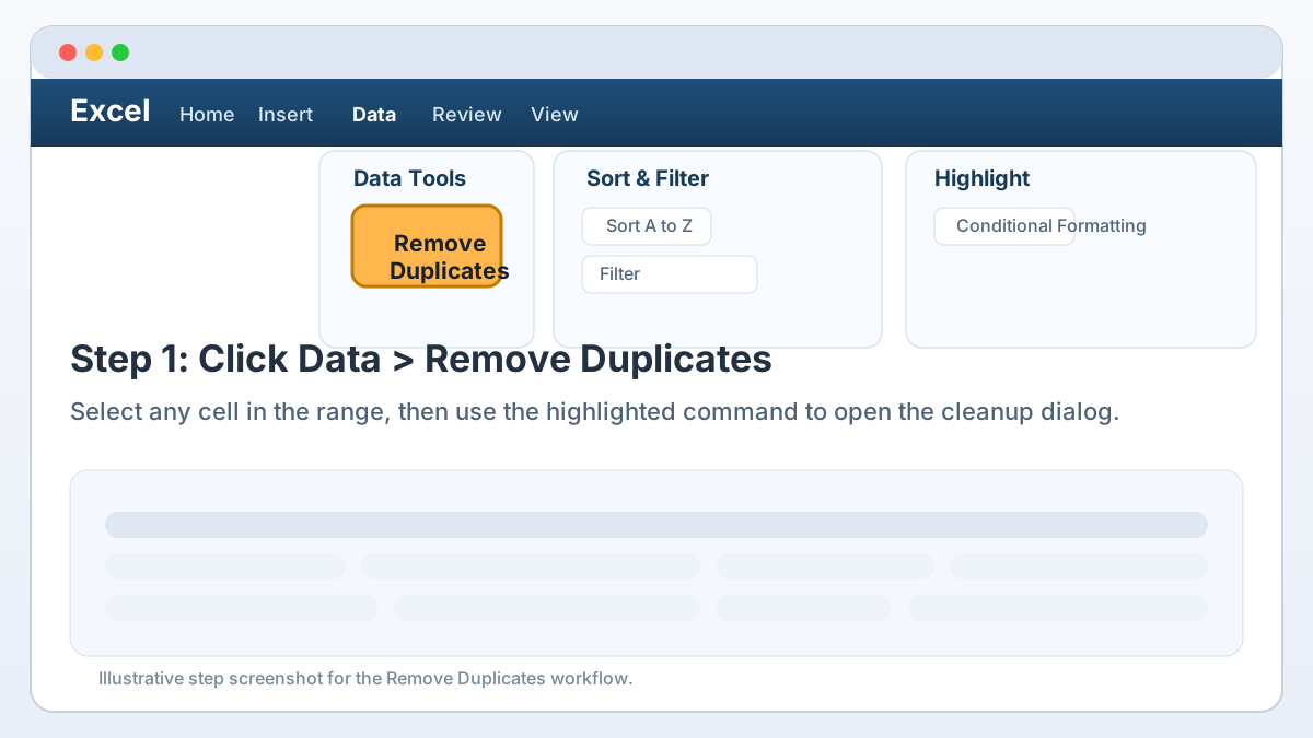
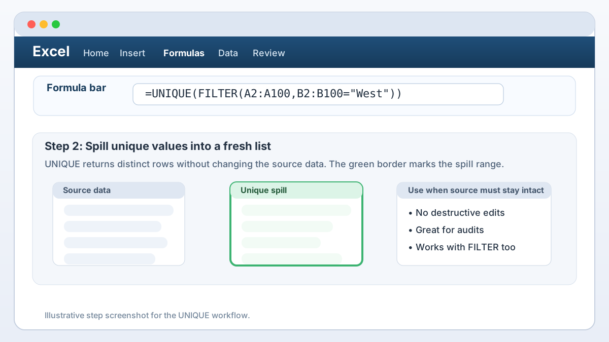
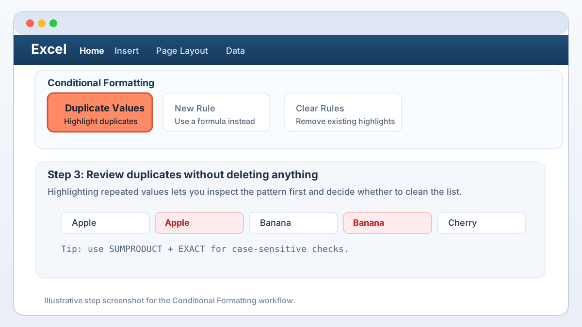
Step screenshots
Use these visual checkpoints when you clean a list in Excel:

Key Takeaways
- Remove Duplicates button is the fastest way to clean existing lists — select your range, click Data > Remove Duplicates, and Excel removes duplicate rows in one click
- UNIQUE function preserves original data while extracting distinct values to a new location, ideal for audit trails and non-destructive analysis
- Conditional Formatting highlights duplicates without deletion, letting you review flagged entries before deciding whether to keep or remove them
- Power Query is ideal for repeatable, refreshable cleanup workflows on imported datasets, with steps you can re-run as new data arrives
How to Remove Duplicates in Excel Using the Built-in Tool
The fastest way to remove duplicates in Excel is Data > Remove Duplicates: select your range, open the dialog, choose which columns define a match, then click OK. Excel keeps the first occurrence of each duplicate set and deletes the rest in place, cleaning list data in seconds.
I reach for this tool whenever I need to delete duplicate rows in Excel from a straightforward list, like a mailing list, a product catalog export, or a set of survey responses. Here is the workflow I follow every time:
- Select any cell inside the data range, or select the full range if you only want to check specific columns.
- Go to the Data tab on the ribbon.
- Click Remove Duplicates.
- Check My data has headers if your first row contains column labels.
- In the dialog box, check the columns that should count toward a match.
- Click OK, and Excel tells you how many duplicate values it removed and how many unique values remain.
This is the same feature most people are describing when they search for how to delete duplicate rows in Excel, because that is exactly what happens once you click OK—matched rows disappear, and only the first instance of each unique record survives.
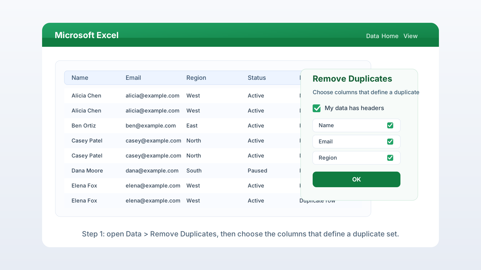
One caveat: Remove Duplicates edits your selection permanently. Before running it on anything you cannot easily rebuild, copy the sheet or save a backup. If you need a repeatable version of this same cleanup, skip ahead to the Power Query section below.
Before you click OK, it also helps to sort the range by whichever field determines priority—date, status, or source—because Excel always keeps the first row it encounters in each duplicate set. If the newest or most complete record happens to appear later in the range, sorting first ensures it survives the cleanup instead of the older duplicate. After the dialog closes, compare the before-and-after row counts and scan the key columns for a quick sanity check.
Using the UNIQUE Function to Remove Duplicates in Excel
The UNIQUE function returns distinct values as a live, non-destructive spill array. Use =UNIQUE(A2:A100) for a single column, or expand the range to include several columns when the combination of fields together defines what counts as a duplicate. Pair it with FILTER to narrow the list by criteria before extracting unique values.
I prefer UNIQUE over Remove Duplicates whenever I need to remove duplicate values in Excel without touching the source data. It builds a fresh list somewhere else in the workbook, so the original range stays intact for auditing or reference.
For a single column, the formula is as simple as it gets:
=UNIQUE(A2:A100)For multiple columns, reference the whole block. Excel treats each row as a unit, so a row is only considered a repeat if every value in that row matches another row exactly:
=UNIQUE(A2:C100)To extract unique values that meet a condition first, wrap the range in FILTER before UNIQUE processes it. For example, this returns unique customer names in column A, but only for rows where the region in column B is “West”:
=UNIQUE(FILTER(A2:A100,B2:B100="West"))If you only need a total rather than a full list, our guide to count unique values walks through wrapping this same pattern in COUNTA. That companion approach answers “how many distinct records do I have” without needing to see the list itself.
Removing Duplicates in Excel Based on One or Multiple Columns
Removing duplicates from one column treats every entry in that column as the whole record, while removing duplicates from multiple columns only deletes a row when every checked column matches another row exactly. Checking more columns makes the match stricter; checking fewer columns makes it looser.
For a single-column scenario, imagine a list of email addresses in column A. Checking only column A in the Remove Duplicates dialog means any repeated email disappears, regardless of what appears in the other columns of that row. This is common when you find duplicates in Excel based on one identifying field, like an order number or an employee ID.
For a multi-column scenario, imagine a customer table with First Name, Last Name, and Email columns. If you check only First Name, Excel might delete legitimate records that just happen to share a common first name. Checking First Name and Last Name together is stricter, and checking all three columns, including Email, is stricter still. The rule to remember:
- Fewer checked columns = broader match = more rows removed
- More checked columns = narrower match = fewer rows removed
I usually start by checking only the columns that represent a true business identifier, such as an email address or invoice number, and I leave notes, timestamps, and comments unchecked so they cannot block a legitimate match.
A good test before you finalize your column selection: ask whether two rows should still collapse into one if a note field or timestamp differs but everything else matches. If the answer is yes, leave that column unchecked. If the answer is no—if that field genuinely changes what the record represents—include it in the match. This one question resolves most of the ambiguity I run into when cleaning imported CRM exports, sales reports, and survey data.
Finding Duplicates Without Deleting Them
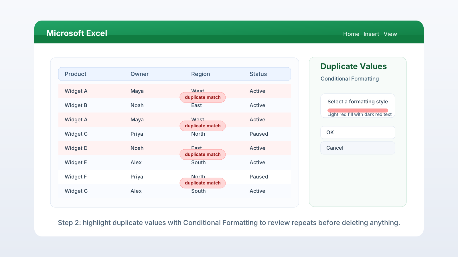
Use Home > Conditional Formatting > Highlight Cells Rules > Duplicate Values to flag repeated entries in color without removing a single row. This lets you find duplicates in Excel first, review them in context, and decide what to keep before running a destructive command like Remove Duplicates.
For formula-based checks, including ways to keep the first match visible or compare several columns, see how to find and highlight duplicates in Excel before you remove any rows.
To set this up:
- Select the range you want to check.
- Go to Home > Conditional Formatting > Highlight Cells Rules > Duplicate Values.
- Choose a fill and font color for the duplicate values.
- Click OK.
Excel immediately highlights every value that appears more than once, so you can scroll through and eyeball the pattern before touching anything.
One limitation of the built-in rule is that it is not case-sensitive—it treats “Apple” and “APPLE” as the same value. If capitalization matters to your business rule, build a custom formula rule instead. Select New Rule > Use a formula to determine which cells to format, then enter a formula that combines EXACT with COUNTIF, such as:
=SUMPRODUCT(--EXACT(A2,A2:A100))>1This counts exact, case-sensitive matches for the active cell against the whole range, so “Apple” and “APPLE” are correctly treated as different values. That extra step matters most for product SKUs, tracking codes, or IDs where letter case is meaningful.
Conditional formatting is also a good sanity check to run right before you click Remove Duplicates. If the highlighted pattern looks different than you expected, it is a sign to revisit which columns you are matching on.
Remove Duplicates from Multiple Sheets or Entire Workbook
Remove Duplicates only works on one selected range at a time, so cleaning several sheets means either consolidating the ranges onto one sheet first or using Power Query’s Append Queries feature to combine everything before you deduplicate. Power Query is the more repeatable option for recurring imports.
If your data is spread across a handful of sheets with the same column structure, the manual path is to copy each sheet’s data into a single staging sheet, then run Remove Duplicates once across the combined range. This works fine for one-off cleanup, but it does not scale well if new sheets get added every month.
For a workbook that grows regularly, I switch to Power Query:
- Load each sheet as a separate query (Data > Get Data > From Table/Range).
- Use Append Queries to stack them into one combined table.
- Apply Remove Duplicates inside the Power Query editor on the combined result.
- Load the cleaned table back into the workbook.
The advantage is that the whole process is saved as a set of steps. When next month’s data arrives in the same shape, you refresh the query instead of repeating the manual copy-and-clean routine. This is also the approach I recommend anytime someone asks how to remove duplicate values in Excel across an entire workbook rather than a single sheet.
If the match logic gets more custom than Remove Duplicates or Power Query can express — fuzzy matching, multi-column tie-breaking rules, or a repeatable script you want to version alongside the workbook — Python in Excel lets you run pandas’ drop_duplicates() directly in a cell using the same worksheet data.
Handling Blanks When Removing Duplicates in Excel
Remove Duplicates treats multiple blank cells in the same column as duplicates of each other, so an entirely blank row can vanish alongside genuine duplicate rows. Filter out blank rows first, or use UNIQUE with FILTER so blanks never enter the distinct list in the first place.
This surprises a lot of people the first time it happens. If your selected range includes three completely blank rows, Excel considers two of them duplicates of the first and removes them, even though nothing was technically “repeated” in a meaningful sense. If you actually need those blank rows preserved as placeholders, exclude them from the selected range before running the command, or handle them separately afterward.
For a formula-based list, the cleaner fix is to filter blanks out before UNIQUE ever sees them:
=UNIQUE(FILTER(A2:A100,A2:A100<>""))This pattern is covered in more depth in our guide to ignore blanks in unique values, which also covers the legacy array-formula version for older Excel builds that do not support dynamic arrays.
If you only need a blank-free count instead of a full list, wrap that same FILTER pattern in COUNTA, which is the same technique used in the count-unique-values guide linked earlier in this article.
Frequently Asked Questions
What is the fastest way to remove duplicates in Excel?
Use Data > Remove Duplicates for a one-click cleanup. This built-in tool instantly scans your selected range, identifies duplicate rows, and removes them in place—keeping only the first occurrence of each unique entry. It works in all Excel versions and is the quickest method for cleaning existing lists.
Does removing duplicates in Excel delete my original data?
Yes, the Remove Duplicates button is destructive—it overwrites your selected range by deleting duplicate rows. If you need to preserve the original data, use the =UNIQUE(range) function instead, which creates a new array of unique values without changing your source data.
How do I remove duplicates based on multiple columns in Excel?
Select your data range, go to Data > Remove Duplicates, then check all columns that define a duplicate. For example, if you check both First Name and Last Name, Excel removes rows only when both columns match exactly, allowing you to keep people with the same first name but different last names.
Can I find duplicates without deleting them in Excel?
Yes. Use Conditional Formatting > Highlight Cells Rules > Duplicate Values to visually flag duplicates in red or another color. This highlights repeating entries without removing them, so you can review duplicates before deciding whether to delete or keep them.
Is there a real cost to leaving duplicate data in a spreadsheet?
Yes. According to Gartner research cited in IBM’s data quality overview, poor data quality costs organizations an average of USD 12.9 million every year (IBM Think — “What is data quality?” accessed 2026-07-10), and duplicate records are a common contributor. Running Remove Duplicates or a UNIQUE-based check before you build a report protects the accuracy of totals and downstream decisions.
