How to Use INDEX MATCH in Excel (Complete Guide)

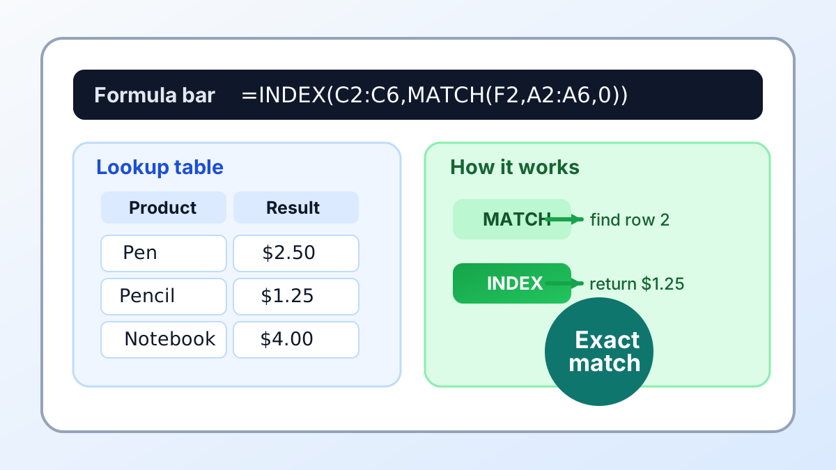
INDEX MATCH is the classic Excel lookup combo when you need a flexible exact match and your workbook cannot rely on XLOOKUP. Microsoft documents MATCH with 3 match modes (-1, 0, and 1), and that exact-match mode (0) is the one most INDEX MATCH formulas use.

If you want the fast version: MATCH finds the position, INDEX returns the value at that position, and together they can look left, right, up, or down depending on how you set the ranges. If you want the broader lookup decision tree first, start with Every Excel LOOKUP Explained. For modern alternatives, compare Excel XLOOKUP vs VLOOKUP and the dedicated Excel XLOOKUP guide.

Stat block: Microsoft Excel worksheets contain up to 1,048,576 rows and 16,384 columns. That scale is one reason lookup formulas matter so much: once a table gets wide or deep, hard-coded column positions become more fragile than position-based lookup logic.

What INDEX MATCH does in Excel

The short answer is that INDEX MATCH separates the job into 2 parts: MATCH finds the row or column number, and INDEX returns the item at that position. Microsoft’s MATCH documentation shows 3 match modes, so the exact-match pattern is both explicit and predictable when you use 0.

The reason people still use it is simple: INDEX MATCH is more flexible than VLOOKUP in older workbooks. VLOOKUP only searches the first column of a range and returns to the right, while INDEX can return from any column or row you point at. That makes the formula easier to adapt when tables move.

A basic example looks like this:

=INDEX($C$2:$C$6,MATCH(F2,$A$2:$A$6,0))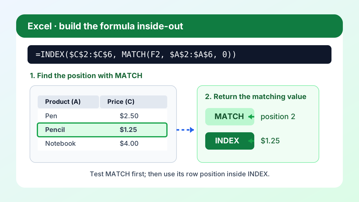

Here is the logic in plain English:

• F2 contains the value you want to find.
• MATCH(F2,$A$2:$A$6,0) returns the row position of that value inside the lookup list.
• INDEX($C$2:$C$6,...) returns the value from the result list at the same position.

If your dataset has unique IDs, product names, or employee numbers, this is the lookup pattern to learn first. It is compact, readable once you know the rhythm, and widely compatible with older versions of Excel that do not include XLOOKUP.

How to build the basic INDEX MATCH formula

The practical way to build INDEX MATCH is to write it inside-out: start with the MATCH part, test the row number, then wrap that result in INDEX. That gives you 2 checks before the formula is even finished, which is why the approach is so easy to troubleshoot.

Start with the lookup value and the lookup range:

=MATCH(F2,$A$2:$A$6,0)

If F2 contains Pencil, this formula returns 2 when Pencil is the second item in A2:A6. That 2 is the position, not the value itself. Once you have that number, you can plug it into INDEX:

=INDEX($C$2:$C$6,MATCH(F2,$A$2:$A$6,0))

A few small habits make the formula much easier to maintain:

• Lock your ranges with $ so the references do not drift when copied.
• Keep the lookup range and return range the same size.
• Use exact match (0) unless you intentionally want approximate results.
• Test MATCH on its own before nesting it inside INDEX.

That last point saves a lot of time. If MATCH returns the wrong position, INDEX will faithfully return the wrong value too. Splitting the formula into 2 parts makes troubleshooting much easier than staring at one long formula and guessing where it went wrong.

How to do a two-way lookup with INDEX MATCH

A two-way lookup is the biggest reason many Excel users learn INDEX MATCH in the first place. Instead of finding just a row, you find both the row and the column, then return the value at the intersection. The pattern uses 2 MATCH functions and 1 INDEX function, so the logic stays precise even in wide tables.

Imagine a table where products run down the rows and months run across the columns. You want the sales value where the product and month intersect. The formula usually looks like this:

=INDEX($B$2:$E$6,MATCH(G2,$A$2:$A$6,0),MATCH(G3,$B$1:$E$1,0))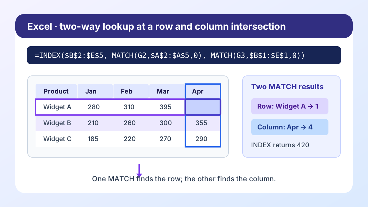

In that formula:

• G2 is the row lookup, such as a product name.
• G3 is the column lookup, such as a month.
• The first MATCH returns the row number.
• The second MATCH returns the column number.
• INDEX returns the value at the intersection of both.

Two-way lookup is especially useful when your report format matches the way people ask questions: “What were April sales for Widget A?” You are not just retrieving a record; you are retrieving a record from a matrix. INDEX MATCH handles that matrix without requiring helper macros or manual rearranging.

If you want to see how this compares with the modern alternative, XLOOKUP can simplify some lookup cases, but it does not fully replace every matrix-style formula. That is why the old pattern still shows up in reporting models, dashboards, and template workbooks.

How to use INDEX MATCH with multiple criteria

Multiple criteria is where INDEX MATCH starts to feel like a power tool. Microsoft’s MATCH docs show exact match mode as 0, and that exact-match behavior is the key ingredient when more than one field has to agree before a value is returned. The challenge is deciding how to combine the criteria.

The simplest route is a helper column. Build a combined key in a new column, then match against that key:

=TEXT(A2,"@")&"|"&TEXT(B2,"@")

If A is product and B is region, the helper column might create values like Widget A|West. Then your lookup becomes:

=INDEX($D$2:$D$100,MATCH(G2&"|"&G3,$C$2:$C$100,0))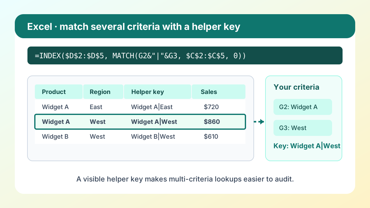

That approach is easy to audit because the criteria are visible in the sheet. It also scales nicely when non-technical teammates will inherit the workbook later.

If you do not want a helper column, you can also build the criteria into the lookup itself with array logic. That version is more advanced and harder to read, so I usually recommend helper columns first unless the workbook design makes them impossible.

A good rule of thumb is this: if multiple people will edit the file, optimize for clarity. If only you will maintain it, optimize for whatever keeps the formula shortest without sacrificing accuracy. In both cases, test the formula on a row you already know is correct before copying it downward.

Common INDEX MATCH problems and when to switch to XLOOKUP

Most INDEX MATCH problems come from 5 places: a mismatched range size, extra spaces in the lookup value, text-versus-number mismatches, duplicate keys, or the wrong MATCH mode. Microsoft documents 3 match modes, so a quick sanity check is to confirm you actually want exact match (0) before troubleshooting anything else.

The fastest debug path is simple:

1. Test MATCH by itself and confirm the row number.
2. Confirm the lookup range and return range are the same size.
3. Check for hidden spaces with TRIM if text should match but does not.
4. Verify numbers are really numbers, not text that only looks numeric.
5. If duplicates exist, decide which one should win before the formula runs.

Example fixes:

=INDEX($C$2:$C$6,MATCH(TRIM(F2),$A$2:$A$6,0))

=INDEX($C$2:$C$6,MATCH(VALUE(F2),$A$2:$A$6,0))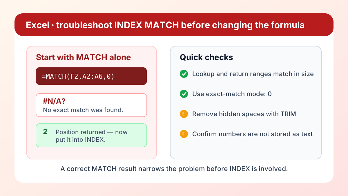

If your workbook supports Microsoft 365, XLOOKUP is often the cleaner choice. It removes the need to combine two functions just to get a basic return value, and it lets you define a friendly not-found result directly in the formula. That makes it easier to read, easier to teach, and easier to audit.

Still, INDEX MATCH remains a good skill to keep. It works in older files, it handles left lookup naturally, and it is still a common pattern in shared corporate workbooks. If you understand both, you can work comfortably across older models and newer templates.

Practical tips for using INDEX MATCH in real workbooks

In large sheets, the biggest reason to be careful with INDEX MATCH is scale: Excel worksheets allow 1,048,576 rows and 16,384 columns, so a small reference mistake can hide in a model for a long time. The safest habit is to make the formula easy to audit before you make it clever.

A few habits help immediately:

• Give the lookup range and result range clear names when the workbook is shared.
• Keep row and column ranges the same size so the position number always maps cleanly.
• Use MATCH alone first, because a wrong position number is easier to spot than a nested formula error.
• Prefer helper columns for multi-criteria lookups when the file will be maintained by other people.
• Use TRIM, VALUE, or TEXT only when you have confirmed that the source data is inconsistent.

If you are building a report for a team, readability usually matters more than shaving off a few characters. A named range like SalesRegion is slower to type than $A$2:$A$100, but it is much easier to understand six months later. The same is true for helper columns: they make the workbook a little wider, but they usually make the logic much more durable.

You should also think about what happens when the table grows. Because INDEX MATCH references positions rather than hard-coded return columns, it is naturally more resilient than VLOOKUP when columns are inserted. That does not make it maintenance-free, though. If the lookup key changes format, or if duplicates appear in the source data, the formula can still return the wrong answer with no visible warning.

That is why the best production workflow is simple: test the formula on a known good row, copy it only after the position output is correct, and keep an eye on the data hygiene around the lookup column. Once those basics are in place, INDEX MATCH becomes a dependable building block instead of a fragile workaround.

FAQ

INDEX MATCH is a 2-function lookup pattern built around exact-position matching, and Microsoft’s MATCH docs show 3 match modes (-1, 0, 1). That makes the FAQ below useful when you are deciding whether to keep the classic formula, switch to XLOOKUP, or build a multi-criteria version.

What does INDEX MATCH do in Excel?

It finds a position with MATCH and returns the value at that position with INDEX. Use it when you need a flexible lookup that can return values from any column or row in a range.

Is INDEX MATCH better than VLOOKUP?

Usually, yes. INDEX MATCH is more flexible because it does not depend on hard-coded column numbers and it can look left as easily as right. VLOOKUP is still fine for simple legacy files.

Can INDEX MATCH look left?

Yes. That is one of its biggest strengths. Since INDEX returns from a separate result range, the return column does not have to sit to the right of the lookup column.

Why use XLOOKUP instead?

Use XLOOKUP when your Excel version supports it and you want the cleanest modern lookup formula. It is easier to read, handles not-found output inside the formula, and covers many cases that previously needed INDEX MATCH.

Does INDEX MATCH work with multiple criteria?

Yes. The easiest approach is a helper column that combines the criteria into one lookup key. You can also use more advanced array-style formulas, but helper columns are usually easier to maintain.

Final takeaway

If you need a reliable exact-match lookup in Excel, INDEX MATCH is still one of the best formulas to know. It is flexible, it works well in older workbooks, and it can handle left lookup, two-way lookup, and multiple criteria without forcing you to reorganize the table.

For a broader lookup strategy, compare it with Every Excel LOOKUP Explained, then decide whether XLOOKUP or INDEX MATCH is the better fit for your workbook. When you understand both, you can choose the simplest formula that still survives real-world spreadsheet changes.