
Analyzing and parsing data in Excel is really a tedious task. If it is not done smartly, then we end up in doing lot of mess. For example, say you have list of email addresses in Excel and you want to extract the extensions of those email addresses. Most of us think of using Text to Columns option and if we proceed using that, then it creates lot of mess. But, Excel expert Oz has a different approach to make it easy for us.
Data Parsing in Excel Using LEN and SUBSTITUTE Functions
Excel MVP Oz explained us the easy way to extract extensions of emails addresses is by using the technique of data parsing using LEN and SUBSTITUTE functions. Let us see, how it can be done step by step.
1 – Finding the Number of Periods
As we all know, LEN () is used to count the number of characters in a cell and SUBSTITUTE () is used to substitute the occurrence of a specific text with the other text you pass to the function as per following syntax,
- SUBSTITUTE (text, old_text, new_text, [instance_num])
- Text – Text where the substitution should take place
- old_text – Text which needs to be replaced
- new_text – Text which needs to be placed in the place of old_text
- [instance_num] – It is optional. If specified, that instance of old_text will be replaced. If not specified, all occurrences of old_text will be replaced
To find the number of periods present in email addresses, select the cell B2 and use the formula =LEN(A2)-LEN(SUBSTITUTE (A2,”.”,””)) and hit enter. Now, you can see the number of periods present in email addresses.
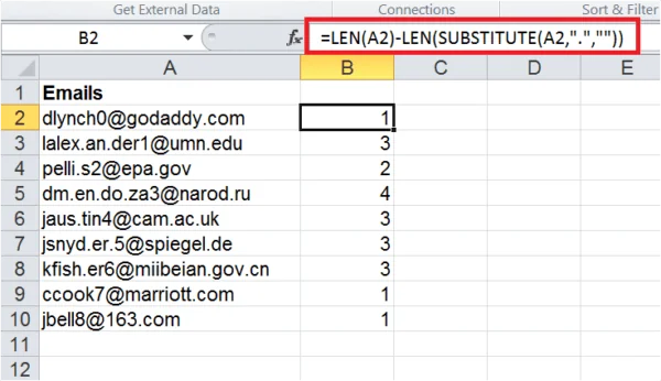
Value in cell ‘B2’ specifies the position of last occurrence of period.
2 – Substitute the last occurrence of period (.) with “^”
In this step, we try to substitute the last occurrence of period (.) with “^”. This is also done using the SUBSTITUTE (), but this time we need to specify the last occurrence (Value in ‘B2’) of period to get it substituted.
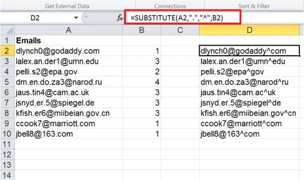
Now, select the cell D2, paste the formula =SUBSTITUTE(A2,”.”,”^”,B2) and hit enter. You can see the formatted text in D2 and drag below to get below cells filled in the same manner.
3 – Find the Position of character “^”
In this step, we will use the FIND () to find the position of the character “^” which we used to substitute period in the previous step.
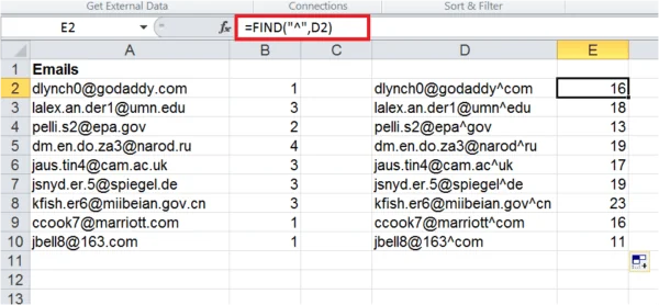
So, select ‘E2’ and use the formula =FIND(“^”,D2) and hit enter. This would give the position of “^” for the text present in column ‘D’.
4 – Extract the extension
This is the final step of extracting the extensions from the email addresses. We use RIGHT () here which meets our requirement.
- RIGHT () Syntax,
- RIGHT (Text, [num_chars])
- Text – string containing the text from which you want to extract the characters
- num_chars – Optional. Specifies the number of characters you want to extract from text from the right end.
Select cell ‘F2’, use the formula =RIGHT(D2,LEN(D2)-E2) and hit enter. You could see the extensions being extracted.
Here,
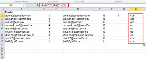
LEN(D2)-E2 gives the number of characters which we want to extract from the right end.
What’s next?
Hope you liked it! Let us know your opinion about this tip. This is really the easy way to parse data in Excel using LEN and SUBSTITUTE functions. If you have anything to add, please do share with us through comments.

Comments (1)
Historical comments preserved from the WordPress archive. Commenting is no longer active.
Good info, i have been using Len() for a long time, but with other functions, good and valuable function.