
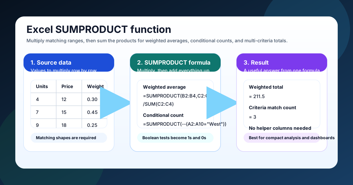
If you want one formula that can handle weighted averages, conditional counts, and multi-criteria totals, SUMPRODUCT is the Excel function to learn first. It is a little less obvious than SUMIF or COUNTIFS, but once you see the pattern, it becomes one of the most flexible tools in the formula toolbox.
The short version is this: SUMPRODUCT multiplies matching items across ranges, then adds the results together. That makes it ideal when you want Excel to do row-by-row math without building helper columns.
Sourced stat block
- Microsoft says SUMPRODUCT returns the sum of the products of corresponding ranges or arrays.
- Microsoft says the array arguments must have the same dimensions, or SUMPRODUCT returns
#VALUE!.- Microsoft warns that a formula like
=SUMPRODUCT(A:A,B:B)multiplies 1,048,576 cells by 1,048,576 cells before adding the results, so full-column references should be avoided.
Key takeaways
SUMPRODUCT is best when one formula needs to multiply aligned values, apply logical tests, and add the surviving results. Use it for weighted calculations or custom criteria logic; use SUMIFS or COUNTIFS for simpler filtering. Keep every array the same size, coerce Boolean tests deliberately, and avoid full-column references in large workbooks.
- SUMPRODUCT is best when you need multiplication plus aggregation in one formula
- It is especially useful for weighted averages and criteria-based totals
- Boolean tests like
A2:A10="West"can be turned into 1s and 0s with-- - Matching range sizes matter more than almost anything else
- Avoid full-column references unless the workbook is tiny or the formula is temporary
What does the SUMPRODUCT function do in Excel?
SUMPRODUCT multiplies corresponding values in equally sized arrays and then adds those row-level products. In one cell, it can calculate revenue from quantity and price, produce a weighted sum, or apply logical tests before totaling results. This multiply-then-add behavior is the foundation for every example in this guide.
That is why SUMPRODUCT sits in the same practical neighborhood as SUMIFS and COUNTIFS, even though the syntax is different. SUMIFS and COUNTIFS filter first and then sum or count. SUMPRODUCT can do the filtering logic inside the multiplication itself.
I like SUMPRODUCT when the worksheet starts to feel like a small model instead of a simple list. It gives you just enough power to stay in a single cell while still keeping the formula readable.
How do you write a basic SUMPRODUCT formula?
Write a basic SUMPRODUCT formula as =SUMPRODUCT(array1,array2), using ranges with identical dimensions. Excel multiplies the first value in each array, repeats that operation row by row, and adds the products. Start with two clean numeric ranges; add logical tests only after the basic calculation returns the result you expect.
=SUMPRODUCT(array1,array2)If the arrays are the same size, Excel multiplies each row pair and adds the results together.
A basic example:
=SUMPRODUCT(B2:B6,C2:C6)If B2:B6 contains quantities and C2:C6 contains unit prices, the formula gives you the total value of those line items.
A few practical notes help a lot here:
- The ranges should line up exactly
- The formula works best when each row represents one record
- Non-numeric entries are treated as zero, which is helpful in some cases and confusing in others
A quick layout example
| Item | Units | Price |
|---|---|---|
| A | 4 | 12 |
| B | 7 | 15 |
| C | 9 | 18 |
The formula =SUMPRODUCT(B2:B4,C2:C4) returns 315 because it calculates 4×12 + 7×15 + 9×18 (48 + 105 + 162).
That row-by-row multiplication is the core idea behind every other SUMPRODUCT trick in this guide.
How do you calculate a weighted average with SUMPRODUCT?
Calculate a weighted average by dividing SUMPRODUCT(values,weights) by SUM(weights). The numerator multiplies each value by its importance and adds those products; the denominator rescales that weighted total into an average. This pattern works for grades, portfolio returns, forecasts, rankings, and any model where observations should not contribute equally.
The pattern is:
=SUMPRODUCT(values,weights)/SUM(weights)Suppose you want a course score, product score, or customer satisfaction score where not every component counts equally. If one test is worth 30% and another is worth 70%, SUMPRODUCT is the cleanest way to combine them.
Example weighted average formula
=SUMPRODUCT(B2:B4,C2:C4)/SUM(C2:C4)If B2:B4 contains scores and C2:C4 contains weights, the formula calculates a weighted result in one cell.
Why this works
The numerator multiplies each score by its weight and adds the products. The denominator adds the weights. Dividing the two gives you the final weighted average.
That means you can use SUMPRODUCT in situations like:
- performance reviews
- grading models
- portfolio returns
- product ranking scores
- sales forecasts with confidence weights
Common weighted-average mistake
The usual mistake is forgetting the denominator. SUMPRODUCT alone gives you a weighted total, not a weighted average. If the weights are supposed to sum to 100%, dividing by SUM(weights) keeps the result on the right scale.
How do you count with multiple conditions using SUMPRODUCT?
For a conditional count with SUMPRODUCT, convert each criterion into a TRUE/FALSE array, coerce the results to 1s and 0s, and add the rows where every required test equals 1. The same pattern supports one condition or several, making it a flexible alternative when COUNTIFS cannot express the logic cleanly.
A comparison like A2:A10="West" gives Excel an array of TRUE and FALSE values. If you prefix that test with --, Excel converts TRUE to 1 and FALSE to 0.
=SUMPRODUCT(--(A2:A10="West"))That formula counts how many cells in A2:A10 equal West.
Counting with two conditions
You can extend the same idea to multiple conditions:
=SUMPRODUCT(--(A2:A10="West"),--(B2:B10="Open"))That returns the count of rows where both conditions are true.
If you prefer to see the logic as multiplication, this equivalent version is often easier to read:
=SUMPRODUCT((A2:A10="West")*(B2:B10="Open"))Both formulas work because TRUE/FALSE values become 1/0 during the calculation.
When SUMPRODUCT is better than COUNTIFS
Use SUMPRODUCT when:
- you want to keep everything in one formula
- you need a custom logical pattern
- you want to combine counting and weighting in one step
- you need a formula shape that COUNTIFS cannot express cleanly
Use COUNTIFS when the task is simply “count rows that meet these conditions.” If the formula gets more mathematical than that, SUMPRODUCT is often the better fit.
How do you sum values when multiple criteria must be true?
To sum values only when multiple criteria are true, multiply each logical test by the numeric range inside SUMPRODUCT. Nonmatching rows become zero, while matching rows retain their values and contribute to the total. This SUMPRODUCT multiple criteria pattern combines filtering and aggregation in one cell without helper columns or nested IF formulas.
A common pattern looks like this:
=SUMPRODUCT((A2:A10="West")*(B2:B10="Open")*C2:C10)If column C contains sales values, the formula sums sales only for rows where region is West and status is Open.
Why this is useful
This pattern is handy when you need a conditional sum but also want the flexibility of full formula logic. It can be easier to debug than nested IF formulas and more expressive than helper-column workarounds.
You can also build OR logic by adding conditions instead of multiplying them. For example, to include West or East:
=SUMPRODUCT(((A2:A10="West")+(A2:A10="East")>0)*C2:C10)That looks a little dense, but the idea is straightforward: if either condition is true, keep the row.
Where this beats SUMIFS
SUMIFS is great when your conditions are straightforward and all behave like filters. SUMPRODUCT is better when you want to combine conditions in more custom ways, such as:
- OR logic across multiple labels
- weighted totals with filters applied
- formulas that need arithmetic alongside logical tests
- counts and sums that share the same formula structure
If you are comparing the two, the Excel SUMIFS Function is the simpler first stop. SUMPRODUCT is the more flexible second stop.
How do you use SUMPRODUCT with text, blanks, and dates?
Use direct equality tests for exact text, <>"" for nonblanks, and numeric comparisons for real Excel dates. SUMPRODUCT does not interpret COUNTIF-style * or ? wildcards inside equality tests. For partial text matches, combine SEARCH with ISNUMBER, then coerce that result before counting or multiplying by a value range.
Text tests
If you want to count or sum a specific label, use a direct text comparison:
=SUMPRODUCT(--(A2:A10="Completed"))For a case-insensitive partial match, use SEARCH with ISNUMBER rather than placing wildcards in an equality test:
=SUMPRODUCT(--ISNUMBER(SEARCH("complete",A2:A10)))SEARCH looks for the text within each cell, ISNUMBER turns each found position into TRUE, and -- converts those results to 1s and 0s for SUMPRODUCT to count.
Blank checks
To count non-blank cells, SUMPRODUCT can work with a simple test such as:
=SUMPRODUCT(--(A2:A10<>""))That is useful when you want a quick count of filled rows, especially in imported lists.
Date tests
Dates are just numbers underneath the formatting, so you can compare them directly if the cells truly contain dates:
=SUMPRODUCT(--(A2:A10>=DATE(2026,1,1)),--(A2:A10<=DATE(2026,1,31)))If date filters behave strangely, the issue is usually that one or more date cells are text instead of real dates.
What are the most common SUMPRODUCT mistakes?
Most SUMPRODUCT mistakes come from mismatched range sizes, full-column references, text stored as numbers, or logical tests that were not coerced consistently. Check those structural issues before rewriting the formula. Matching dimensions and bounded ranges prevent the most common errors, while deliberate -- or multiplication makes Boolean behavior easier to understand and audit.
1. Range sizes do not match
Microsoft is explicit here: the arrays must have the same dimensions. If one range is B2:B10 and another is C2:C12, SUMPRODUCT will not guess what you meant.
Fix: make the ranges identical in height and width.
2. Full-column references slow things down
Microsoft warns against A:A and B:B in SUMPRODUCT because the function evaluates every cell in the column. That is unnecessary work in most workbooks.
Fix: use a bounded range like A2:A5000 instead.
3. Text numbers are treated like text, not numbers
If numbers were imported as text, SUMPRODUCT may treat them as zeros or simply fail to produce the result you expected.
Fix: convert the source values to numbers first.
4. You forgot the double unary or the multiplication coercion
Logical comparisons like A2:A10="West" create TRUE/FALSE arrays. Sometimes Excel handles them fine in multiplication, but if you are counting rather than summing, the -- coercion keeps the behavior consistent.
Fix: use -- when you need a clean numeric count.
5. You expected SUMPRODUCT to act like SUMIFS
SUMPRODUCT can mimic SUMIFS in many cases, but it is not the same function. SUMIFS is a filter-and-sum tool. SUMPRODUCT is a math-and-aggregation tool.
Fix: choose the function that matches the task instead of forcing one to behave like the other.
When should you use SUMPRODUCT instead of SUMIFS or COUNTIFS?
Use COUNTIFS for straightforward counts, SUMIFS for straightforward conditional sums, and SUMPRODUCT when the formula must combine criteria with arithmetic, weighting, or custom OR logic. SUMPRODUCT is more flexible, but that flexibility can reduce readability. Choose the simplest function that expresses the rule clearly and remains easy for others to audit.
- Use COUNTIFS when you need a clean count with one or more straightforward criteria
- Use SUMIFS when you need a clean sum with one or more straightforward criteria
- Use SUMPRODUCT when the logic is more mathematical, more custom, or both
That makes SUMPRODUCT especially good for:
- weighted averages
- weighted scores
- ranking models
- conditional totals with OR logic
- counts and sums that depend on several logical tests at once
- formulas that need to stay in one cell without helper columns
If you are building reports that mostly count rows between two values, the Excel COUNTIF Between Two Numbers guide is the better companion. If you are building a formula that needs sums plus conditions, SUMPRODUCT usually gives you more control.
SUMPRODUCT formula example: multi-criteria sales total
For a multi-criteria sales total, multiply the Region test, the Status test, and the Sales range inside SUMPRODUCT. Rows that fail either test become zero; rows that pass both retain their sales value. Excel then adds only those surviving values, producing a conditional total in one formula without a helper column.
Here is a complete SUMPRODUCT formula example you can copy directly into your own worksheet. Let’s say you have three columns:
- Region
- Status
- Sales
You want the sales total for rows where Region is West and Status is Open. If you only need a plain running total with no conditions attached, the Excel SUM Formula guide covers that simpler case.
The formula is:
=SUMPRODUCT((A2:A100="West")*(B2:B100="Open")*C2:C100)What happens inside the formula
- Excel checks whether each region equals West
- Excel checks whether each status equals Open
- Excel multiplies the two logical arrays together
- Excel multiplies the result by the Sales column
- Excel adds the surviving sales values together
That sequence is why SUMPRODUCT is so useful. You are not just counting or summing blindly. You are explicitly telling Excel which rows survive and which rows do not.
A second example: weighted sales score
Suppose you want a score where revenue is weighted by margin quality:
=SUMPRODUCT(C2:C100,D2:D100)/SUM(D2:D100)If column C contains ratings and column D contains weights, the formula returns the weighted average score.
This is one of the simplest and most useful ways to turn a messy worksheet into a decision-ready number.
Related reading
The most useful companion guides depend on whether your next task is a plain total, a criteria-based sum, or a criteria-based count. Start with SUM for uncomplicated addition, SUMIFS for conventional conditional totals, and COUNTIF for range counts. Return to SUMPRODUCT when weighting or custom Boolean logic makes those simpler functions restrictive.
- Excel SUM Formula
- Excel SUMIFS Function
- Excel COUNTIF Between Two Numbers
- Excel COUNTIF Function: Complete Guide
Frequently asked questions
These answers summarize the decisions readers most often make with SUMPRODUCT: when to use it, how to calculate a weighted average, how to count several criteria, why errors appear, and whether full-column references are sensible. The same five topics also appear in the page’s structured FAQ data, keeping machine-readable guidance consistent with the visible article.
What does SUMPRODUCT do in Excel?
It multiplies corresponding values in ranges or arrays and then adds the products together. That makes it ideal for weighted totals, weighted averages, and conditional counting.
How do I use SUMPRODUCT for a weighted average?
Use =SUMPRODUCT(values,weights)/SUM(weights). The numerator gives you the weighted total, and the denominator turns that into an average.
Can SUMPRODUCT count rows with multiple criteria?
Yes. Wrap your logical tests in -- or multiply them together, and SUMPRODUCT will count the rows where the tests return TRUE.
Why does SUMPRODUCT give me #VALUE!?
The most common cause is mismatched range sizes. Microsoft says the array arguments must have the same dimensions.
Should I avoid full-column references in SUMPRODUCT?
Yes, in most cases. Microsoft warns that full-column references force SUMPRODUCT to process every cell in the column, which can slow the workbook down.
