How to Find & Highlight Duplicates in Excel

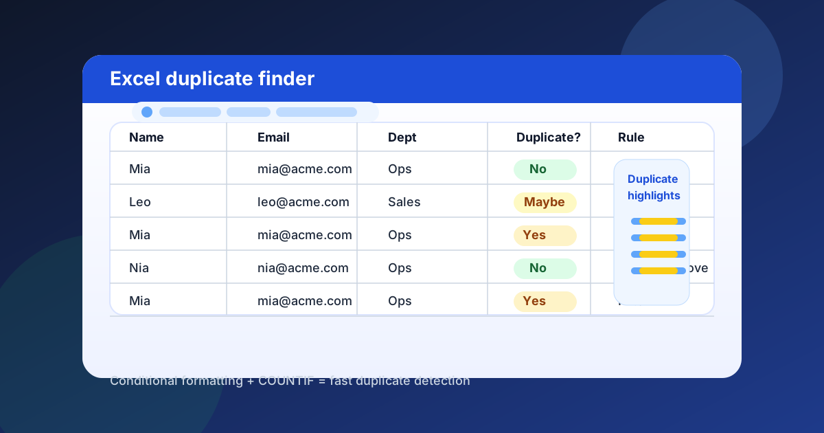
If you need the short version: use Conditional Formatting with a COUNTIF formula to highlight duplicate values, then use Data > Remove Duplicates only after you’ve made a copy of the sheet. That gives you a fast visual check first and a safer cleanup second.

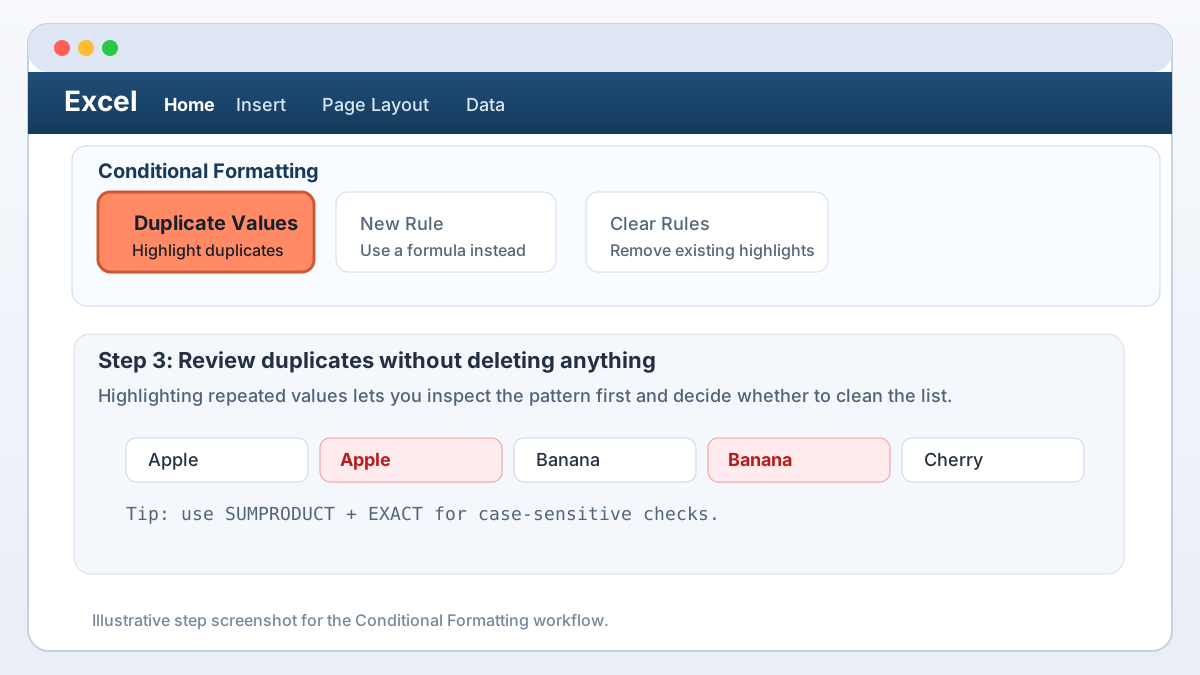
Key takeaways

• Highlight duplicates first, remove them second. Seeing the pattern before deleting anything prevents accidental data loss.
• COUNTIF is the simplest duplicate detector. It works for one column, repeated values, and “second copy onward” highlighting.
• A helper column is the best fix for multi-column matches. If a record is only a duplicate when several fields match, build a combined key first.
• Clean the text before you compare it. Extra spaces, invisible characters, and inconsistent case are the usual reasons duplicate checks feel “wrong.”
• Keep the original sheet untouched. Copy the data or work in a duplicate workbook before removing anything.

Stat block: IBM’s data quality guide says poor data quality costs organizations an average of USD 12.9 million each year, and duplicate data is one of the problems that contributes to that cost. Source: IBM Think — “What is data quality?” (accessed 2026-07-10).

The fastest way to find duplicates in Excel

The quickest way to spot duplicates is with Conditional Formatting, which I also use in my broader Excel conditional formatting guide and my walkthrough on how to color code in Excel.

Here’s the version I use most often for a single column of names, IDs, or email addresses:

1. Select the data range, for example A2:A1000.
2. Go to Home > Conditional Formatting > New Rule.
3. Choose Use a formula to determine which cells to format.
4. Enter this formula:

=COUNTIF($A$2:$A$1000,A2)>1

5. Pick a fill color and click OK.

That formula says: count how many times the current cell value appears in the whole list. If the count is more than 1, Excel formats it.

A couple of practical notes:

• Lock the full range with $A$2:$A$1000.
• Leave the final cell reference as a relative reference (A2) so Excel can evaluate each row correctly.
• If your data extends beyond row 1000, expand the range or use a larger range than you expect to need.

If I’m working with imported customer data, I usually turn the range into an Excel Table first. Tables make the rule easier to maintain when rows are added later.

How to highlight duplicates in Excel with a formula

If you want a more precise rule than the preset duplicate option, use a custom formula. I prefer this approach because it gives me control over the exact range and the exact visual style.

A clean general-purpose rule looks like this:

=COUNTIF($A$2:$A$1000,A2)>1

Use it when you want every repeated value to light up, including the first copy.

If you only want repeat occurrences to highlight, not the first instance, use a running range instead:

=COUNTIF($A$2:A2,A2)>1

That version is especially useful when I’m cleaning a list and want to preserve the first record while flagging every later copy.

When I choose formula-based highlighting

I use formula-based highlighting when:

• the built-in duplicate rule is too blunt,
• I want a different format for first vs later matches,
• I need to include or exclude blank cells,
• or I’m comparing values across a custom range.

For example, if blank cells are triggering false positives in your sheet, you can exclude them with a slightly stricter rule:

=AND(A2<>"",COUNTIF($A$2:$A$1000,A2)>1)

That tells Excel not to highlight empty rows.

How to find duplicates across two or more columns

Single-column checks are easy. Multi-column duplicate detection is where most people get stuck.

Let’s say a row is only a duplicate when first name + last name + department all match. In that case, I build a helper column and join the fields into one comparison key.

For example:

=A2&"|"&B2&"|"&C2

Fill that down, then run the duplicate check on the helper column.

If you’re on Microsoft 365, you can also use TEXTJOIN:

=TEXTJOIN("|",TRUE,A2:C2)

That makes it easier to combine several columns without writing a long concatenation chain by hand. If you need a deeper refresher on string assembly, the Excel concatenate guide covers the basics and the delimiter variations.

A better pattern for messy imported data

When I know the source file is messy, I normalize the text before I compare it:

=LOWER(TRIM(CLEAN(A2)))

That combination removes extra spaces, strips many invisible characters, and makes text comparisons case-insensitive.

If the match depends on several columns, I apply the same cleaning step to each part before concatenating them.

That one habit saves a lot of time because many “duplicate” problems are really just formatting problems.

How to highlight only the second copy and later copies

This is one of the most useful duplicate tricks in Excel because it keeps the original record visible.

Use this conditional-formatting formula:

=COUNTIF($A$2:A2,A2)>1

What it does:

• The first time a value appears, the running count is 1, so nothing is highlighted.
• The second time it appears, the count becomes 2, so Excel formats that row.
• Every later repeat is also highlighted.

I like this approach when I’m reviewing a CRM export, an address list, or a lead sheet where the first instance should stay untouched.

If you’re using this on a large worksheet, keep the selected range tight. Conditional formatting is powerful, but it’s still a calculation rule, and unnecessarily large ranges can slow things down.

How to remove duplicates safely in Excel

Once you’ve highlighted the duplicates and confirmed the pattern, removing them is straightforward.

Use this workflow:

1. Make a copy of the worksheet or the workbook.
2. Select the data range.
3. Go to Data > Remove Duplicates.
4. Choose the columns that define a duplicate.
5. Click OK.

That’s the safest path because Excel deletes rows immediately. If you’re not sure whether a column should be part of the comparison, copy the sheet and test on the duplicate version first.

My rule for choosing columns

I usually include only the fields that define true sameness.

For example:

• A customer list might compare email address only.
• An order list might compare order ID and line item ID.
• A person list might compare first name, last name, and date of birth.

If you include too many columns, real duplicates slip through. If you include too few, you’ll delete rows that were actually distinct.

A better alternative for “keep everything, just unique values”

If you need a clean unique list without deleting anything from the source, use a separate sheet and extract unique values there. In many cases, that is a better workflow than modifying the raw data directly.

How to avoid false positives when Excel finds duplicates

Most duplicate-checking problems come from dirty input, not from Excel itself.

Here are the fixes I use most often:

1) Remove extra spaces

A trailing space makes two values look identical to the eye but different to Excel.

Use:

=TRIM(A2)

2) Strip non-printing characters

Imported CSVs and copied web data sometimes contain invisible characters.

Use:

=CLEAN(A2)

3) Normalize case

If you want case-insensitive matching, wrap the cleaned value in LOWER():

=LOWER(TRIM(CLEAN(A2)))

4) Check the data type

A number stored as text can behave differently from a number stored as a value. The same thing happens with dates.

If duplicate detection feels inconsistent, confirm the type before you compare the cells.

5) Watch for merged cells and formatted blanks

Merged cells and empty-looking cells with formatting can make the range hard to reason about. If the result looks strange, unmerge the sheet or copy the data into a clean range first.

How I handle duplicates when I’m comparing two lists

Sometimes the real task is not “find duplicate values in one list” but “find which values in List A also appear in List B.”

For that, I often use a comparison column or a lookup pattern.

If you want a deeper comparison workflow, the Excel VLOOKUP compare two columns guide is a good companion read.

A simple duplicate check between two lists can look like this:

=COUNTIF($B$2:$B$1000,A2)>0

That tells you whether the value in A2 exists anywhere in the second list.

I like this when I’m merging mailing lists, matching exported reports, or checking whether a cleaned list already exists in another workbook.

What I do after I find duplicates

Once the duplicates are highlighted, I decide what kind of duplicate I’m actually dealing with:

• True duplicate: same record entered more than once.
• Near duplicate: same entity, but one field differs.
• Dirty duplicate: same record, but with extra spaces, punctuation, or formatting noise.

That distinction matters because each one needs a different fix.

For true duplicates, I usually remove the extra rows. For near duplicates, I merge or reconcile the conflicting fields. For dirty duplicates, I clean the source text first and then run the duplicate check again.

If the sheet is getting hard to read after all the highlighting, I’ll often freeze the header row or reorganize the list before doing the cleanup. In longer workflows, it can also help to unsort the sheet after testing so I’m back to the original order before I publish or share the file.

A quick pre-delete checklist

Before I delete anything, I run through a short checklist:

• Save a copy of the workbook first. A duplicate cleanup is only truly safe when you have a rollback path.
• Confirm the comparison columns. Ask whether a duplicate is defined by one field or by a combination of fields.
• Scan for blanks and dirty text. Empty rows, invisible spaces, and odd punctuation can make the result look wrong.
• Sort or filter the data if it helps you review the pattern. Sometimes grouping identical values together makes the duplicate logic much easier to verify.
• Check your counts before and after cleanup. If you expect 500 rows to stay and 20 to disappear, make sure the numbers match.

I find this quick pause saves a lot of time. It also keeps me from deleting records that looked repetitive but were actually unique.

If the workbook is shared with other people, I also leave a note in the sheet or the file comments so the next person knows what comparison rule I used. That is especially helpful when the duplicate definition is business-specific, such as one customer per email, one order per invoice number, or one contact per company plus department.

FAQ

What is the easiest way to find duplicates in Excel?

The easiest method is Conditional Formatting with a COUNTIF formula. It takes less than a minute to set up and gives you an immediate visual result.

Can Excel highlight duplicates automatically?

Yes. Excel’s built-in duplicate rule under Conditional Formatting can highlight repeated values automatically as soon as you apply it.

Can I find duplicates across multiple columns?

Yes. The easiest approach is to create a helper column that combines the fields you want to compare, then run the duplicate check on that helper key.

Why does Excel think two values are different when they look the same?

Usually because of hidden spaces, non-printing characters, inconsistent case, or a value being stored as text instead of a number.

Should I use Remove Duplicates right away?

Not on the original sheet. I always highlight first, verify the pattern, and copy the file before deleting anything.

Can I use formulas instead of the Remove Duplicates tool?

Yes. Formulas are better when you want a live, auditable view of the duplicate logic. The Remove Duplicates tool is better when you want a one-time cleanup.

If you want, I can also turn this into a step-by-step tutorial for duplicates across two columns, highlighting duplicates in a table, or removing duplicate rows while keeping the latest record.