
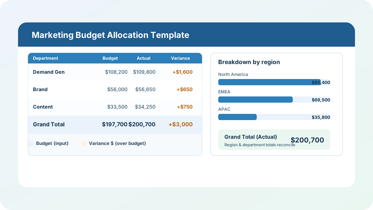
Every marketing budget consolidation I’ve run into starts the same way: three or four department heads each have their own spreadsheet, someone copies and pastes all of them into one master tab before the finance review, and by the second review cycle nobody’s numbers match anymore because two people edited the same shared tab at the same time. This marketing budget allocation template fixes that by giving each department its own sheet to own, then rolling every department’s line items up automatically — by department, by region, by month, and by product line — on a separate Summary sheet that nobody needs to touch by hand.
Download the marketing budget allocation template — it’s a plain .xlsx, no macros, no external data connections, and no sign-up. Open it in Excel or Google Sheets and start replacing the sample departments and line items with your own.
Who is this template for?
I built this for the marketing operations lead or CMO who’s consolidating budget requests from multiple teams — demand gen, brand, content, whatever your org chart looks like — into one document ahead of a finance or leadership review. If you’ve spent a review cycle reconciling three departments’ spreadsheets by hand, cross-checking a region total against a month total to make sure nothing got double-counted or dropped, this template does that reconciliation automatically instead of asking you to redo it every month.
What’s in the workbook, sheet by sheet
The workbook ships with five sheets, in this exact order:
- Instructions — setup steps and a clean-room disclosure: every formula, layout, and sample figure in this workbook was authored from scratch for Excel.TV. No vendor template, workbook, or dataset was downloaded, inspected, or adapted to build it.
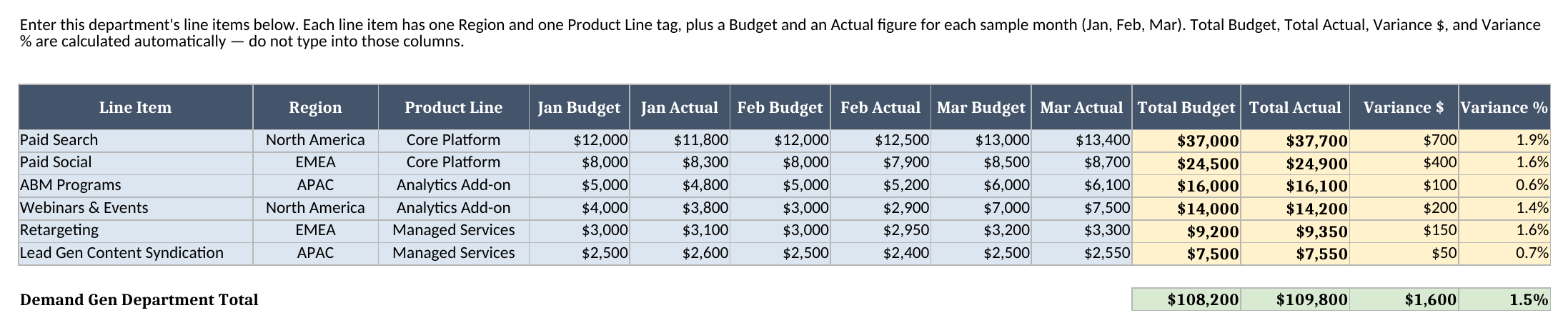
- Demand Gen — this department’s own line items: paid search, paid social, ABM programs, webinars, retargeting, and lead-gen content syndication in the sample, each tagged with a Region and a Product Line, with Budget and Actual figures for Jan, Feb, and Mar.
- Brand — the Brand department’s line items, in the same layout as Demand Gen: brand campaigns, sponsorships, PR, creative production, and brand research in the sample.
- Content — the Content department’s line items, in the same layout again: blog and SEO content, video production, case studies, localization, and editorial tools and licensing.
- Summary — the consolidated view: Department Totals, then automatic breakdowns by Region, by Month, and by Product Line, each with a “Total (check)” row that re-sums the breakdown and should always match the Grand Total.
The required inputs are each department’s own line items — the Region tag, the Product Line tag, and the monthly Budget/Actual figures — entered on that department’s own sheet. The main outputs are Summary’s Department Totals, Region, Month, and Product Line breakdowns, which recalculate the instant anyone changes a figure on any of the three departmental sheets.
How do I set up my own departments and line items?
- Open Demand Gen, Brand, and Content and replace the sample line items with your own team’s budget requests, one row per line item.
- For each line item, set Region to one of North America, EMEA, or APAC, and Product Line to one of Core Platform, Analytics Add-on, or Managed Services — both columns use dropdown validation, and Summary’s breakdowns depend on these tags matching exactly.
- Enter each line item’s Budget and Actual figures for Jan, Feb, and Mar. Total Budget, Total Actual, Variance $, and Variance % are calculated automatically per line item, and each department’s own Department Total row at the bottom of its sheet sums the whole department.
- To add a new line item, insert a row above a department’s Department Total row, copy the Total Budget/Total Actual/Variance formulas down into it, and extend that sheet’s own Department Total SUM range to include the new row.
- Open Summary and confirm the Department Totals table, and each breakdown’s “Total (check)” row, look right for your data.
How does the automatic Summary roll-up actually work?
This is the mechanic that makes this template different from copy-and-pasting three departments’ numbers into one tab. Every cell on Summary’s Department Totals table is a direct cross-sheet reference to that department’s own Department Total row — for example, Demand Gen’s Actual is ='Demand Gen'!K11, pointing straight at the SUM formula already sitting on the Demand Gen sheet. Nothing is retyped, so there’s no chance of a transcription error between a department’s sheet and the consolidated view.
The Region, Month, and Product Line breakdowns go one step further: each one uses SUMIF (or plain SUM for the month columns, since each department sheet already has one column per month) across all three departmental sheets at once, added together into a single formula. The North America row’s Actual figure, for instance, is three SUMIF calls added together — one reading Demand Gen’s Region column, one reading Brand’s, one reading Content’s — each summing that department’s Total Actual column wherever Region equals “North America.” Change a single line item’s region on any department’s sheet, and that one formula picks it up without anyone touching Summary at all.

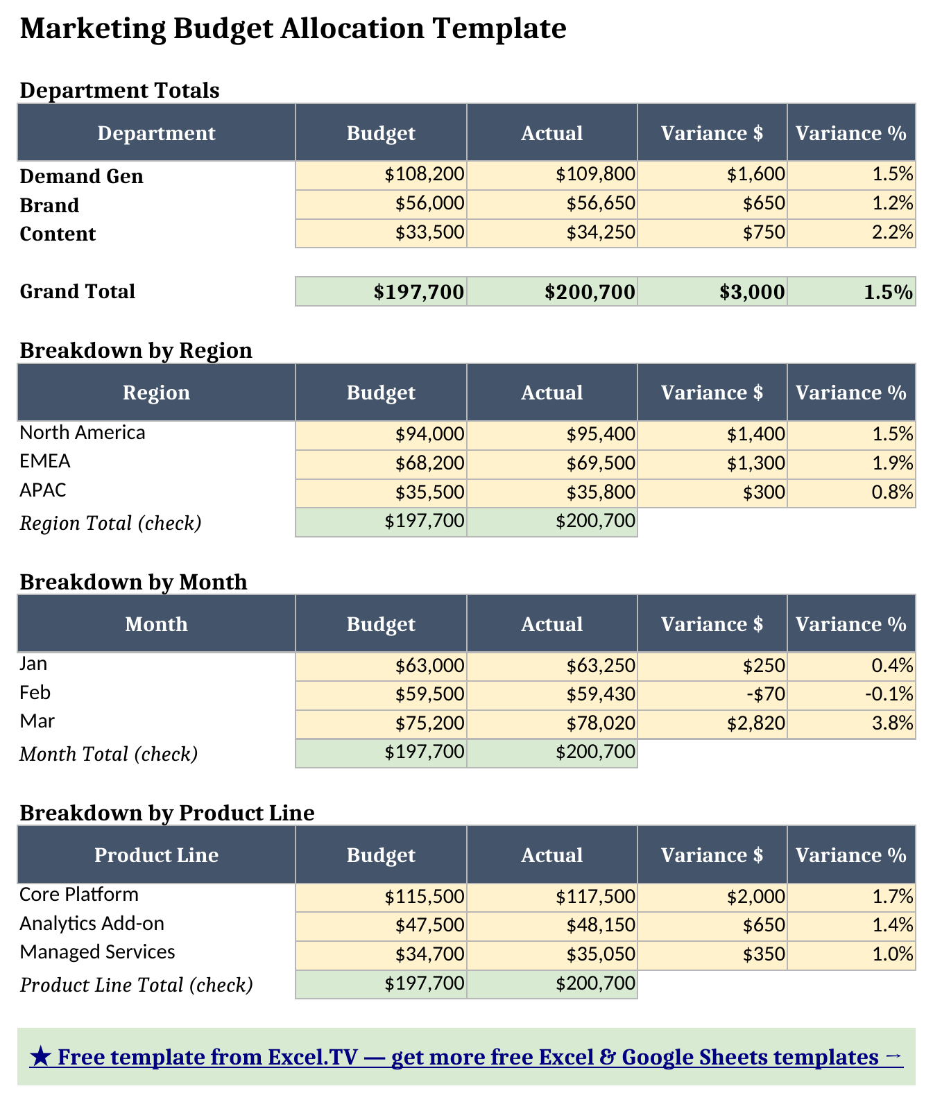
I built a reconciliation check directly into the breakdown tables for exactly this reason: every breakdown table on Summary — Region, Month, and Product Line — ends in a “Total (check)” row that re-sums the breakdown’s own rows. If that check row ever stops matching the Grand Total after you’ve added or removed line items, it means a departmental sheet’s own SUM/SUMIF range needs to be widened to include the new rows — you’ll see it immediately instead of discovering it during a finance review. Here’s the Region breakdown from the sample workbook, straight from a full formula recalculation, showing the check row matching the Grand Total exactly:
| Region | Budget | Actual | Variance $ | Variance % |
|---|---|---|---|---|
| North America | $94,000 | $95,400 | +$1,400 | 1.5% |
| EMEA | $68,200 | $69,500 | +$1,300 | 1.9% |
| APAC | $35,500 | $35,800 | +$300 | 0.8% |
| Region Total (check) | $197,700 | $200,700 |
Worked example: department totals from the sample workbook
Here’s the full Department Totals table for the sample workbook, pulled straight from Summary after a full formula recalculation:
| Department | Budget | Actual | Variance $ | Variance % |
|---|---|---|---|---|
| Demand Gen | $108,200 | $109,800 | +$1,600 | 1.5% |
| Brand | $56,000 | $56,650 | +$650 | 1.2% |
| Content | $33,500 | $34,250 | +$750 | 2.2% |
| Grand Total | $197,700 | $200,700 | +$3,000 | 1.5% |
Every department ran slightly over budget in the sample data, and the Grand Total — $200,700 actual against $197,700 budgeted, a $3,000 variance — is simply the sum of the three department rows above it, which is itself simply the sum of every department’s own line items. That’s the whole point of the design: the Grand Total isn’t a separately-maintained number that can drift from the departments underneath it, it’s the same figures rolled up twice, once by department and once (as shown above) by region, and both roll-ups land on exactly $200,700.
The Month breakdown tells a story the Department Totals table can’t: Jan came in $250 over budget, Feb actually came in $70 under budget, and Mar — the month with the sample’s biggest spend, including a fundraising-style sponsorship push on Brand’s sheet — ran $2,820 over, a 3.75% variance. None of that seasonal detail is visible from department totals alone, which is exactly why a real budget consolidation needs more than one way to slice the same numbers.
How do I use this in Google Sheets?
Open Google Sheets, choose File > Import > Upload, select the downloaded .xlsx, and pick “Insert new sheet(s).” Every formula in this workbook — SUM, SUMIF, IF, IFERROR, and ABS — is natively supported in Google Sheets, so nothing needs to be rewritten, including the cross-sheet SUMIF formulas driving the Region, Month, and Product Line breakdowns. The dropdown data validation on each departmental sheet’s Region and Product Line columns also carries over automatically.
If you’d rather skip the download-and-import step entirely, use this one-click copy link: make a copy of the Marketing Budget Allocation Template in Google Sheets. Google will prompt you to save it to your own Drive, and from there it behaves identically to the Excel version — same sheets, same departmental line items, same Summary roll-ups.
Limitations to know before you rely on this
A few things are worth knowing before you hand this to your finance team:
- Each line item gets exactly one Region and one Product Line. This template doesn’t split a single line item’s spend proportionally across two regions or two product lines — if a campaign genuinely spans both, split it into two line items instead.
- The sample period is one quarter (Jan, Feb, Mar), not a full year. Extending it to twelve months means adding a Budget/Actual column pair per month on each departmental sheet, extending every line item’s Total Budget/Total Actual formulas to include the new columns, and adding matching rows to Summary’s Breakdown by Month using the same SUM pattern already there.
- Adding or removing a line item requires extending that sheet’s own SUM range, and if a department’s row range changes, Summary’s SUMIF ranges for that sheet need updating too — the breakdowns don’t auto-expand on their own, which is exactly what the “Total (check)” rows are there to catch.
- Three departments (Demand Gen, Brand, Content) is a working example, not a hard limit. Add a fourth departmental sheet the same way the first three were built, and add one row to Summary’s Department Totals table referencing it.
- No macros, no external connections. Everything here is a native formula. That’s deliberate — it’s what keeps the workbook portable between Excel and Google Sheets with zero substitutions.
I’d rather you know these limitations going in than discover one the week before a budget review. Once each department’s line items are entered on its own sheet, the Summary roll-ups take care of themselves.
Download the marketing budget allocation template and swap in your own departments whenever you’re ready.
