
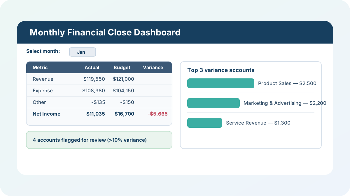
I build a lot of monthly reporting packages for finance teams that don’t have a dedicated FP&A system, and the same problem comes up every time: actuals live in one file, budget lives in another, and by the time someone reconciles them by hand, the “monthly close” has eaten most of a week. This finance dashboard excel template is my answer to that — one workbook where actuals and budget flow into a variance analysis and a one-page dashboard automatically, built around a real monthly financial close, for whatever month you pick.
Download the finance dashboard excel template — it’s a plain .xlsx, no macros, no external data connections, and no sign-up. Open it in Excel or Google Sheets and start replacing the sample numbers with your own.
Who is this template for?
I built this for a small finance or accounting team running a monthly close on their own chart of accounts — the kind of team that’s outgrown a single “budget vs. actual” tab but doesn’t need (or can’t yet justify) a BI tool. If you can export actuals and a budget by account and by month, you can drop them into this workbook and get a dashboard out the other end. It also works well as a teaching example if you want to see INDEX/MATCH, SUMIF, and a month-selector dropdown working together in one connected model.
What’s in the workbook, sheet by sheet
The workbook ships with six sheets, in this exact order, because each one depends on the sheet before it:
- Instructions — a short setup guide plus a clean-room disclosure: every formula, layout, and sample figure in this workbook was authored from scratch for Excel.TV. No vendor template, workbook, or dataset was downloaded, inspected, or adapted to build it.
- Chart of Accounts — the master list of 15 sample accounts (code, name, type, category, and notes). Everything else in the workbook looks up from this list, so it’s where you add, remove, or rename accounts.
- Actuals Input — your closed-period actual amounts, one row per account, one column per month.
- Budget Input — your budgeted amounts, laid out the same way as Actuals Input.
- Variance Analysis — a fully calculated sheet that pulls actual vs. budget for every account, for whichever month is selected on the Dashboard.
- Dashboard — the one-page summary: a month selector, revenue/expense/net income vs. budget, a count of accounts flagged for review, and the three largest dollar variances.
The required inputs are just two things per account per month: an actual amount on Actuals Input and a budgeted amount on Budget Input. The main outputs are the Dashboard’s key metrics, the flagged-account count, and the top-3 variance ranking — all of which recalculate the instant you change the month selector or edit an input cell.
How do I set up the monthly financial close dashboard?
- Open Chart of Accounts and replace the sample account list with your own — keep each Account Code unique, since every lookup in the workbook keys off it.
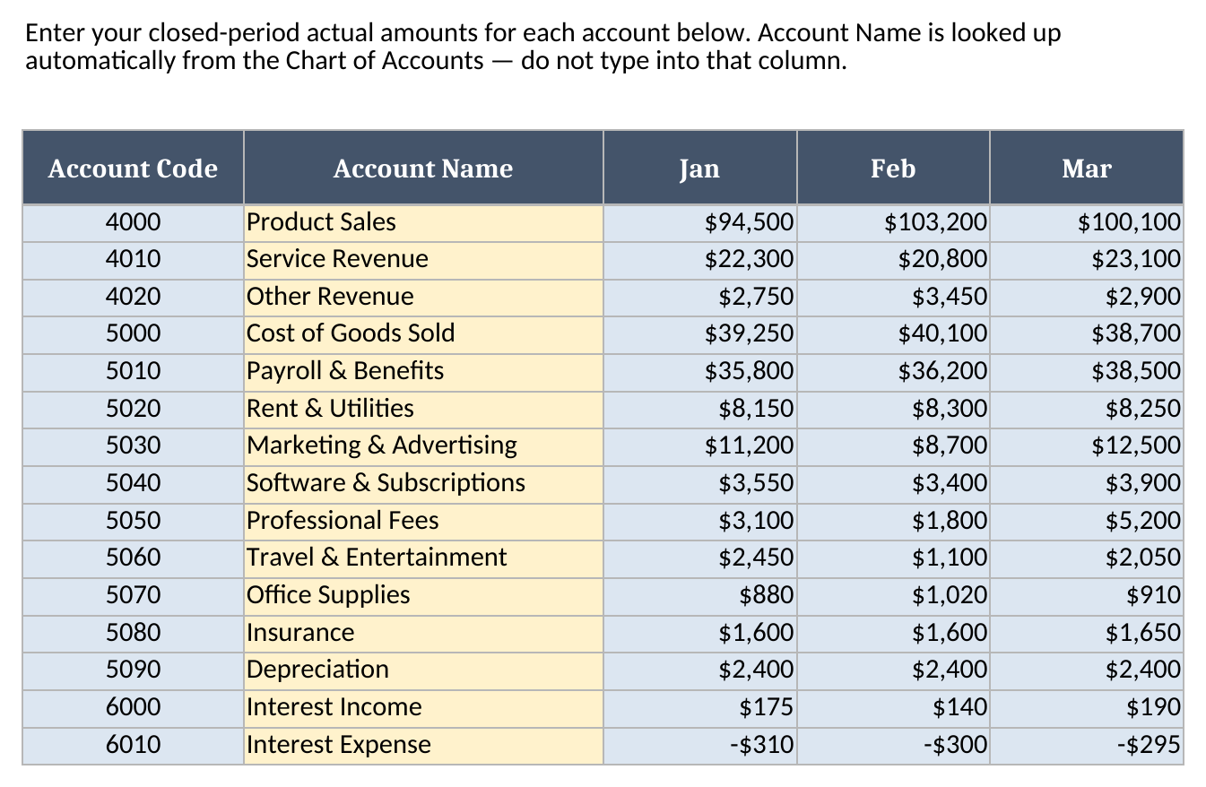
- Open Actuals Input and enter your actual amounts for each account, for each closed month. Don’t type into the Account Name column; it’s a formula that looks up the name from Chart of Accounts automatically.
- Open Budget Input and enter your budgeted amounts in the same account order.
- Go to Dashboard and use the month selector dropdown to choose which month to review.
- Check Variance Analysis for the account-level detail behind the Dashboard’s totals.
Because Account Name on both input sheets is an INDEX/MATCH formula rather than typed text, a typo in an account code shows up immediately as “(unknown account)” instead of silently mismatching later.
How the variance analysis flags accounts for review
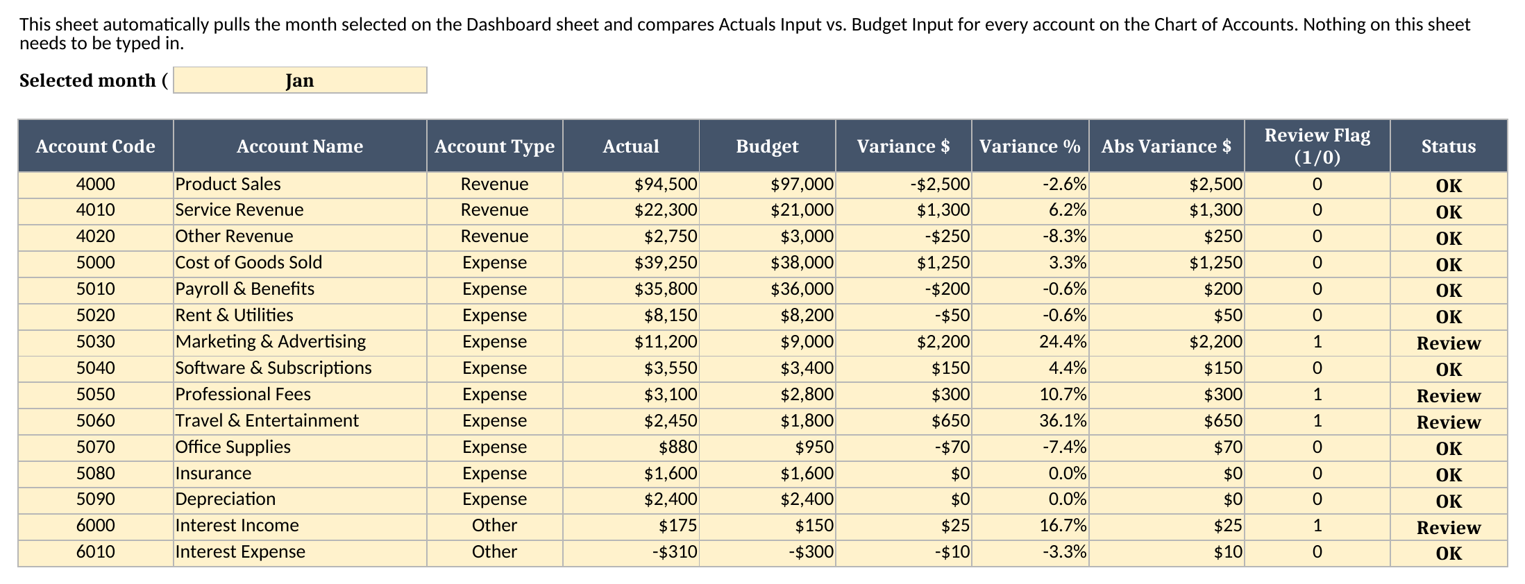
Variance Analysis is where the real work happens, and you never type into it. For every account it pulls the selected month’s actual and budget with a two-way INDEX/MATCH — matching the account code down the rows and the month across the columns — then calculates a dollar variance, a percentage variance, and an absolute-value variance. A Review Flag column marks any account more than 10% off budget in either direction, and a Status column turns that flag into a plain “Review” or “OK.”
Looking at January in the screenshot below, Marketing & Advertising came in at $11,200 against a $9,000 budget — a 24.4% variance — so it’s flagged. Professional Fees and Travel & Entertainment are flagged too, along with Interest Income, which puts January at four flagged accounts total.
Worked example: closing January, February, and March
I built three months of synthetic sample data into the template specifically so you can see the dashboard react to a real close cycle instead of a single static snapshot. Here’s what the Dashboard shows for each month, pulled straight from the workbook:
| Month | Revenue (Actual / Budget) | Expense (Actual / Budget) | Net Income Actual | Net Income Budget | Net Income Variance | Accounts Flagged |
|---|---|---|---|---|---|---|
| Jan | $119,550 / $121,000 | $108,380 / $104,150 | $11,035 | $16,700 | -$5,665 (-33.9%) | 4 |
| Feb | $127,450 / $123,500 | $104,620 / $104,500 | $22,670 | $18,850 | $3,820 (20.3%) | 3 |
| Mar | $126,100 / $126,200 | $114,060 / $110,450 | $11,935 | $15,610 | -$3,675 (-23.5%) | 3 |
January closed under budget on Net Income mostly because Marketing & Advertising overspent by $2,200 and Product Sales came in $2,500 light — those are the two largest dollar variances that month, with Service Revenue’s $1,300 shortfall rounding out the top three. February flips the story: Product Sales beat budget by $4,200, which is the single biggest swing in any of the three months, and it’s enough to push Net Income $3,820 over budget even with Cost of Goods Sold running $1,100 hot. March lands back below budget, driven by a $2,500 Marketing & Advertising overage and a $1,500 miss on Payroll & Benefits.
This is exactly what I want a monthly close report template to do: let one number — Net Income variance — tell you whether the month needs a closer look, and let the top-3 ranking tell you where to look first, without opening a second file.
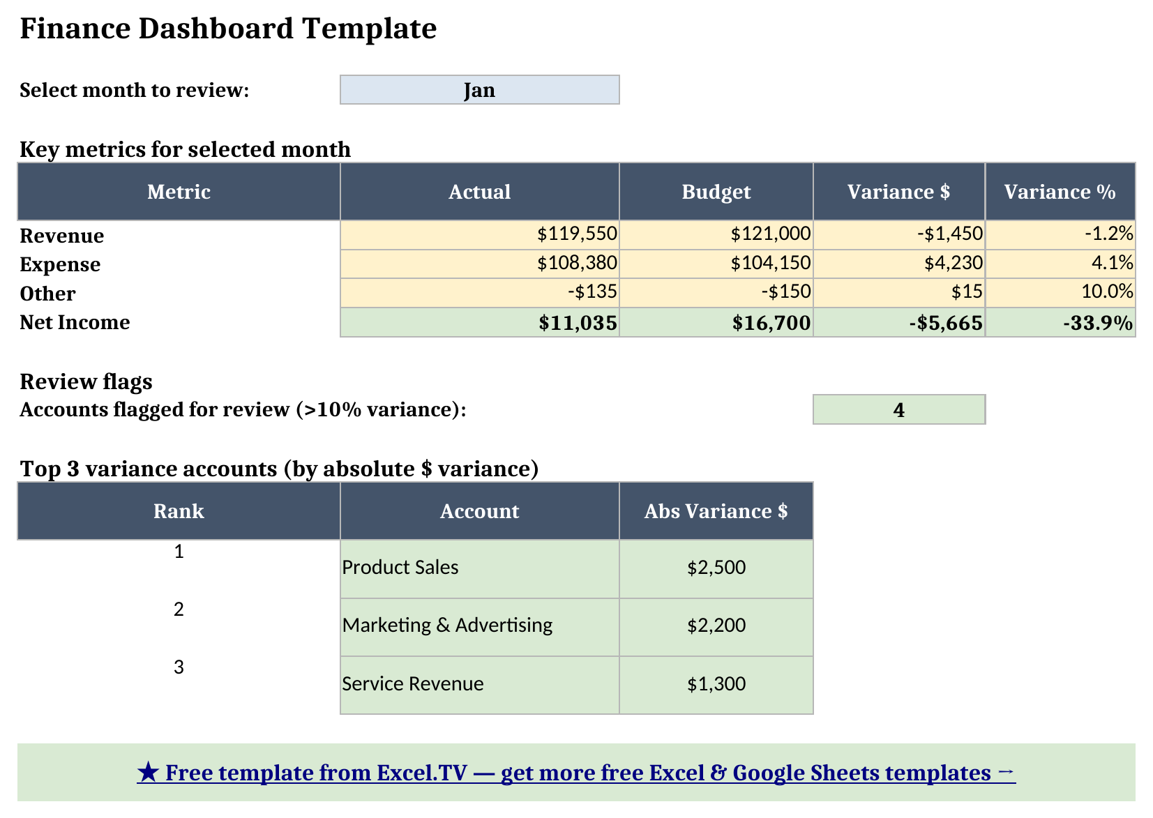
Grab the finance dashboard excel workbook if you want to flip the month selector yourself and watch these numbers update live.
How do I use this in Google Sheets?
Google Sheets is a first-class destination for this excel dashboard template, not an afterthought. Open Google Sheets, choose File > Import > Upload, select the downloaded .xlsx, and pick “Insert new sheet(s).” Every formula in this workbook — SUM, SUMIF, IF, IFERROR, INDEX, MATCH, ABS, ROUND, and LARGE — is natively supported in Google Sheets, so nothing needs to be rewritten, and the month-selector dropdown’s data validation carries over with it.
If you’d rather skip the download-and-import step entirely, use this one-click copy link: make a copy of the Finance Dashboard Template in Google Sheets. Google will prompt you to save it to your own Drive, and from there it behaves identically to the Excel version — same sheets, same formulas, same month selector.
If you’re assembling a fuller business dashboard excel template for a monthly reporting package and haven’t set up the budget side yet, my budget spreadsheet walkthrough covers building that input from scratch; and if the budget you’re closing against is a marketing line rather than a full P&L, my marketing budget allocation template is built for that narrower case.
Limitations to know before you rely on this
A few things are worth knowing before you put real numbers in:
- Every sheet needs the same account order. The workbook assumes each account code is unique and appears exactly once, in the same set of rows, on Chart of Accounts, Actuals Input, and Budget Input. Insert a row in one sheet without inserting it in the others and the lookups will mismatch.
- “Other” is added, not subtracted, into Net Income. Net Income is
Revenue − Expense + Other, so a non-operating expense filed under Account Type “Other” — Interest Expense in the sample data — has to be entered as a negative number. Enter it as a positive number by mistake and it will inflate Net Income instead of reducing it. Non-operating income accounts, like Interest Income, stay positive as usual. - Ties in the top-3 ranking aren’t broken. The
LARGE+MATCHpattern that ranks the three biggest variances returns the first matching account if two accounts tie exactly on absolute dollar variance. That’s an inherent limitation of this lookup pattern without an added tie-breaker column. - The 10% review threshold is a fixed sample value. Change the flag formula on Variance Analysis directly if your close process uses a tighter or looser threshold.
- No macros, no external connections. Everything here is a native formula. That’s deliberate — it’s what keeps the workbook portable between Excel and Google Sheets with zero substitutions.
I’d rather flag these limitations up front than have you discover them mid-close. Once you know the account-order rule and the Other-sign rule, the rest of the workbook takes care of itself.
