
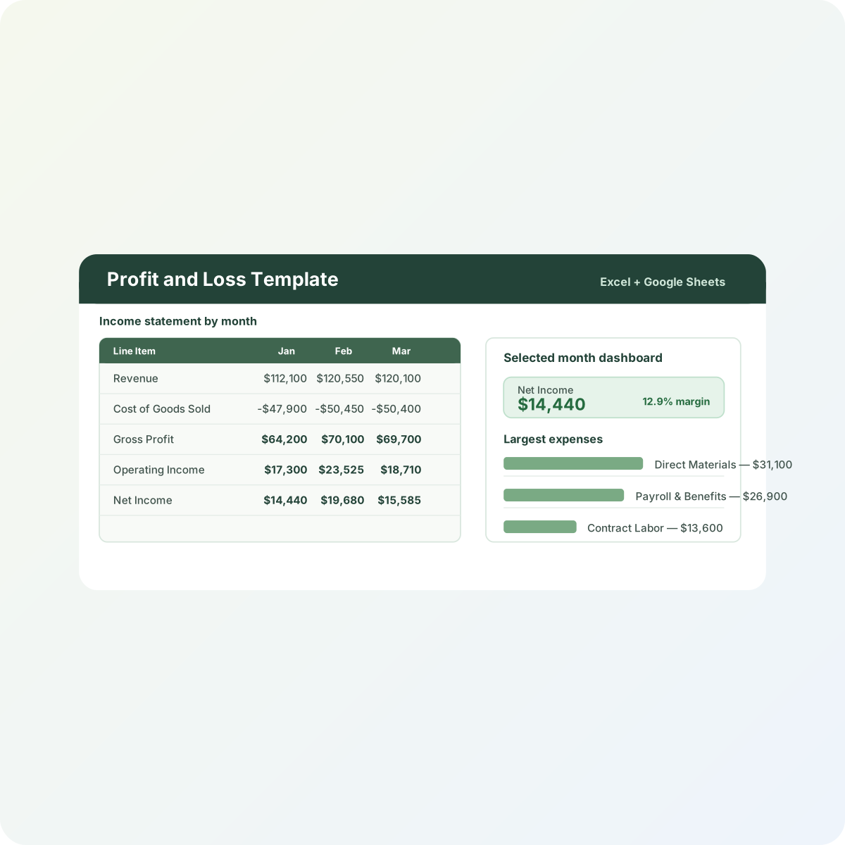
I have seen a lot of small-business P&Ls that are technically correct and still hard to use. The owner exports a ledger, sorts it by account, adds a few subtotals, and then starts moving numbers around until the income statement looks presentable. That works once. It does not work when you need to compare January to February, explain why net income moved, or hand the file to someone else without a 20-minute warning about which cells not to touch. This profit and loss template excel workbook is built to avoid that problem: transactions go in one place, account types drive the P&L, and the dashboard updates from the statement instead of from hand-entered summary numbers.
Download the profit and loss template - it is a plain .xlsx, no macros, no external data connections, and no sign-up. Open it in Excel or import it into Google Sheets and replace the synthetic sample data with your own accounts and monthly transactions.
Who is this template for?
I built this for the person who needs a practical income statement template spreadsheet, not a textbook definition of profit. That might be a founder closing the books before a board update, a bookkeeper preparing a monthly management report, a consultant teaching a client how revenue flows down to net income, or a small finance team that wants a cleaner bridge between a transaction export and a one-page dashboard.
The workbook is intentionally simple. It is not an accounting system, and it is not trying to replace your general ledger. Its job is narrower: take a monthly transaction list with account codes and amounts, map those accounts into P&L sections, and produce a clean monthly profit and loss statement with a few trend and dashboard views on top. If you already have accounting software, you can export a transaction or trial-balance style report and use this as the management-reporting layer. If you are still building your first reporting file, the sample data gives you a working model to study before you put real numbers in.
I also wrote it as a teaching workbook. You can inspect the formulas and see the logic clearly: account names and account types are pulled with INDEX/MATCH, P&L sections are summed with SUMIFS, margin rows use IFERROR, and the dashboard’s largest-expense list uses LARGE with MATCH. Nothing is hidden behind a macro or add-in.
What’s in the workbook, sheet by sheet
The workbook ships with six sheets in this exact order:
- Instructions - a setup guide, clean-room disclosure, color legend, Google Sheets import note, limitations, and workbook CTA.
- Chart of Accounts - the master account list: Account Code, Account Name, Account Type, Category, and Notes. Account Type is the important field because it tells the P&L whether a transaction belongs in Revenue, COGS, Operating Expense, Other Income, Other Expense, or Tax Expense.
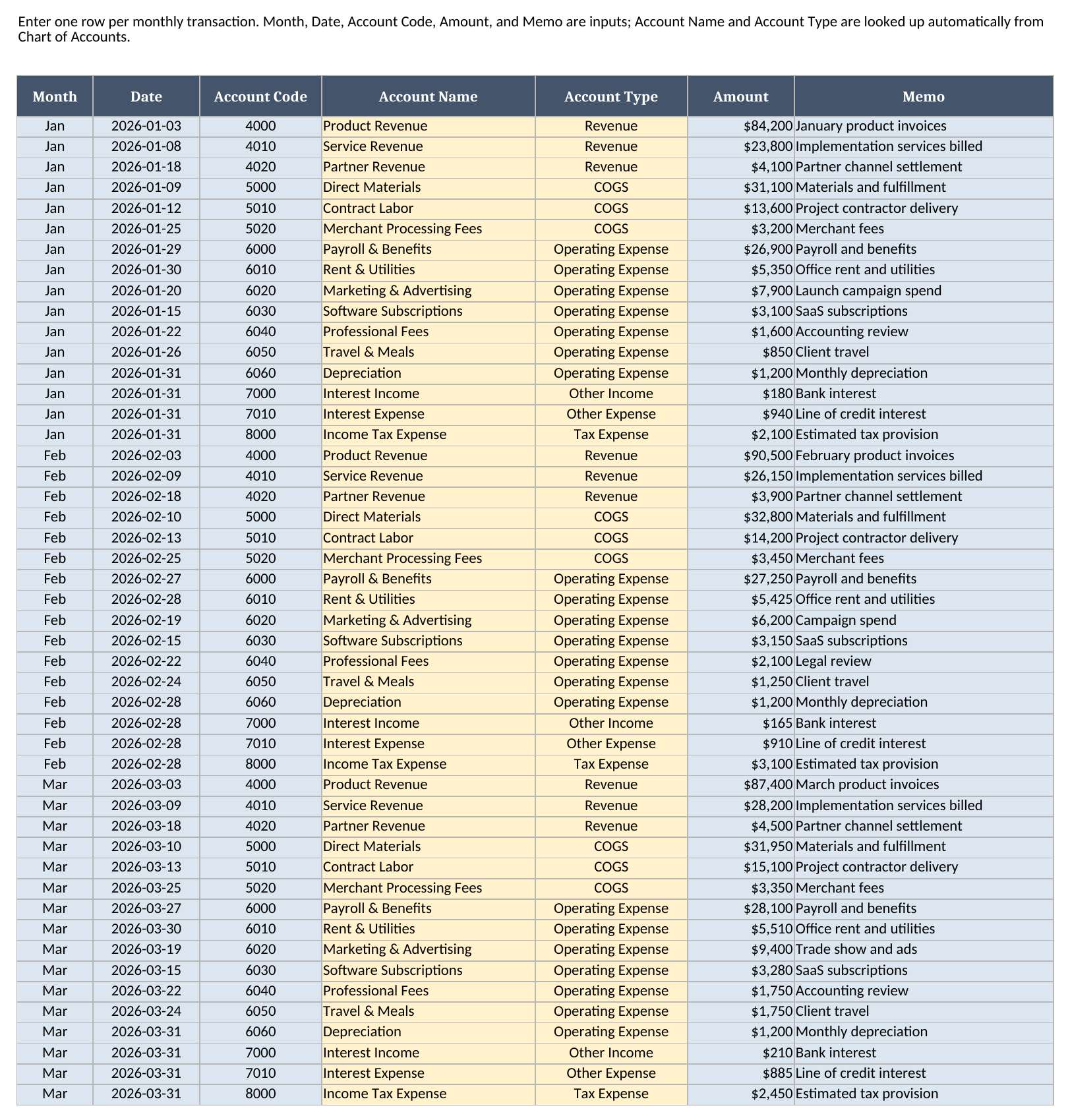
- Monthly Transactions - the editable input ledger. You enter Month, Date, Account Code, Amount, and Memo. Account Name and Account Type are calculated from Chart of Accounts so the P&L can summarize consistently.
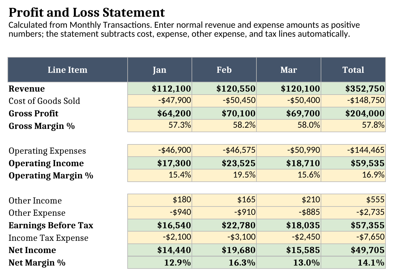
- P&L - the calculated profit and loss statement by month. It shows Revenue, Cost of Goods Sold, Gross Profit, Gross Margin, Operating Expenses, Operating Income, Operating Margin, Other Income, Other Expense, Earnings Before Tax, Income Tax Expense, Net Income, and Net Margin.
- Trend Analysis - the same key lines arranged for month-to-month review: revenue, revenue growth, gross profit, gross margin, operating income, operating margin, net income, and net margin.
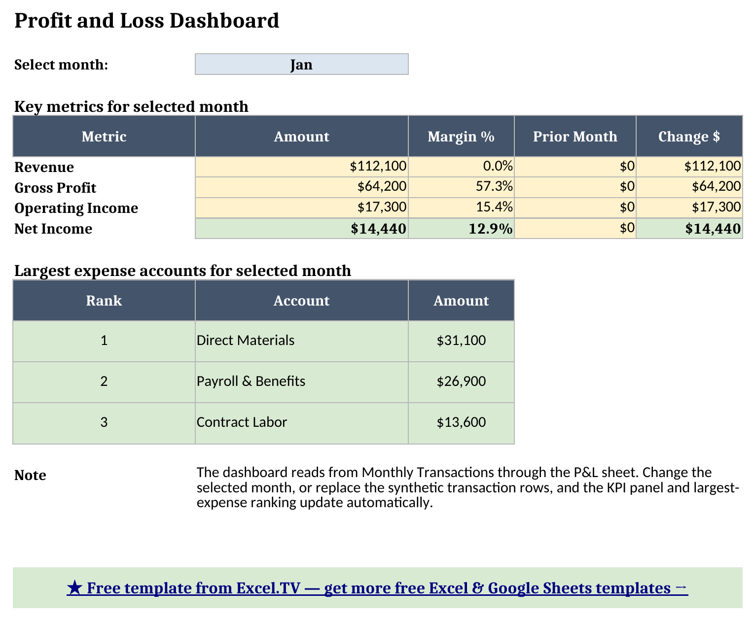
- Dashboard - a one-page selected-month summary with a month dropdown, headline KPIs, prior-month comparison, and the three largest expense accounts.
The required inputs are your account list and your monthly transactions. The main outputs are the P&L statement, margin percentages, month-to-month trend rows, and dashboard KPIs. Once the accounts are mapped correctly, the workbook does not need you to retype subtotals every month.
How do I set up the profit and loss template?
- Open Chart of Accounts and replace the sample account codes and names with your own. Keep each Account Code unique.
- Assign each account one of the workbook’s supported Account Types: Revenue, COGS, Operating Expense, Other Income, Other Expense, or Tax Expense.
- Open Monthly Transactions and replace the sample rows with your own entries. Use one row per transaction or one summarized row per account per month, depending on the level of detail you want.
- Enter normal revenue and expense amounts as positive numbers. The P&L sheet subtracts COGS, operating expenses, other expenses, and tax expense automatically.
- Review P&L and Trend Analysis for the calculated monthly statement and margin movement.
- Open Dashboard and use the month selector to review one month at a time.
The Account Name and Account Type columns on Monthly Transactions are formula-driven on purpose. If you type an account code that does not exist on Chart of Accounts, the lookup returns “(unknown account)” or “(unknown type)” instead of quietly filing the transaction under the wrong heading. That is one of the small spreadsheet safeguards I like because it catches a common mistake close to where the mistake is made.
How the P&L formulas work
The core of the workbook is not complicated, and that is deliberate. The P&L does not summarize by account name directly. It summarizes by Account Type, which is what lets you change account names, add a new marketing account, or split a revenue account later without rewriting the statement layout.
For example, the January Revenue line uses a SUMIFS pattern that says: sum Amount from Monthly Transactions where Month is Jan and Account Type is Revenue. Cost of Goods Sold uses the same idea, but the P&L multiplies the result by negative one so it displays as a deduction. The same treatment applies to Operating Expense, Other Expense, and Income Tax Expense. That is why the setup instructions tell you to enter normal expenses as positive numbers. The statement controls the sign based on the account type.
Gross Profit is then simple arithmetic: Revenue plus the displayed COGS line. Since COGS is shown as a negative number, the formula reads like the statement: revenue plus a deduction. Operating Income adds Gross Profit and Operating Expenses. Earnings Before Tax adds Operating Income, Other Income, and Other Expense. Net Income adds Earnings Before Tax and Income Tax Expense.
The margin rows are there because I do not like P&Ls that force you to evaluate every change in dollars only. A $5,000 increase in revenue means something different when revenue is $40,000 than when it is $400,000. Gross Margin % is Gross Profit divided by Revenue, Operating Margin % is Operating Income divided by Revenue, and Net Margin % is Net Income divided by Revenue. Each one is wrapped in IFERROR so an empty or zero-revenue month returns 0.0% instead of throwing a divide-by-zero error.
Worked example: January through March
I included three months of synthetic data so you can see the template behave like a real monthly P&L instead of a static one-month statement. These figures came from the generated workbook after a LibreOffice recalculation pass, which is the same check I use before quoting workbook numbers in the article.
| Month | Revenue | Gross Profit | Operating Income | Net Income | Net Margin |
|---|---|---|---|---|---|
| Jan | $112,100 | $64,200 | $17,300 | $14,440 | 12.9% |
| Feb | $120,550 | $70,100 | $23,525 | $19,680 | 16.3% |
| Mar | $120,100 | $69,700 | $18,710 | $15,585 | 13.0% |
January is a good baseline month: $112,100 of revenue, $47,900 of COGS, and $46,900 of operating expenses land at $14,440 of net income. February improves because revenue rises to $120,550 while marketing spend drops from the January launch campaign, so net income reaches $19,680 and net margin expands to 16.3%. March revenue stays almost flat at $120,100, but trade-show and advertising spend pushes operating expenses higher, so net income falls back to $15,585 even though gross profit is still strong.
That is exactly the kind of movement I want a P&L template to make obvious. If I only looked at revenue, February and March look almost identical. Once the expenses and margins are visible, the story changes: March did not have a revenue problem as much as it had an operating-spend problem. The Dashboard reinforces that by ranking the largest expense accounts for the selected month. In January, Direct Materials, Payroll & Benefits, and Contract Labor are the three largest expense lines. If you switch the dropdown to March, Marketing & Advertising moves up because of the trade-show spend in the sample data.
How do I use this in Google Sheets?
This is also a profit and loss template google sheets users can work with. Download the .xlsx, open Google Sheets, choose File > Import > Upload, select the workbook, and choose Insert new sheet(s). After import, keep the same sheet order and test the Dashboard month selector. The formulas used in this workbook - SUM, SUMIFS, IF, IFERROR, INDEX, MATCH, ABS, ROUND, LARGE, and arithmetic - are native to Google Sheets, so no substitutions are required.
I did not include a one-click Google Sheets /copy URL in this release because the Drive REST publishing credentials were not configured in the build environment available for this task. I would rather state that plainly than invent a link. The Phase 1 delivery is the tested .xlsx import path above: download the workbook, import it into Google Sheets, and save the imported spreadsheet to your own Drive.
One practical Google Sheets note: after import, check the data validation dropdowns on Chart of Accounts, Monthly Transactions, and Dashboard. They are standard list validations and should carry over, but I still like confirming the month selector before using a newly imported workbook for reporting.
How this differs from a generic income statement spreadsheet
Most generic income statement template excel files are laid out like a statement first and a model second. You type revenue into the Revenue row, type expenses into the expense rows, and hope you remember which month was updated. That is fine for a one-time presentation, but it is fragile as a recurring monthly process.
This workbook starts one level lower, with transactions and account mapping. I prefer that structure because it leaves an audit trail. When Net Income changes, you can go back to Monthly Transactions and see which rows caused the change. When an account is misclassified, you fix the Account Type on Chart of Accounts instead of hunting through a statement full of pasted numbers. When you want the dashboard to show a different month, you change one dropdown instead of rebuilding the summary section.
There is a tradeoff. A transaction-driven workbook takes a few more minutes to set up than a blank statement tab. You have to care about account codes. You have to be consistent about month labels. But once that structure is in place, the P&L, trend view, and dashboard all reuse the same inputs. That is the difference between a spreadsheet that looks finished and a spreadsheet that can survive next month’s close.
If you are building a wider reporting package, my finance dashboard excel template adds budget-versus-actual variance and review flags. If you are starting with the planning side instead of actuals, my budget spreadsheet walkthrough is the better next stop.
Limitations to know before you rely on this
A few things are worth knowing before you put real numbers in:
- This is a management P&L, not accounting software. It does not post journal entries, enforce debits and credits, reconcile bank accounts, or close periods.
- Account Type drives the statement. If an account is misclassified on Chart of Accounts, the P&L will faithfully put it in the wrong section. Check the account mapping before trusting the output.
- Normal expenses should be positive. COGS, operating expenses, other expenses, and tax expense are subtracted by formula. Enter a negative expense only for a real credit, refund, or reversal.
- The month list is fixed to Jan, Feb, and Mar in the sample workbook. You can extend it, but add months deliberately across Monthly Transactions, P&L, Trend Analysis, and the Dashboard selector.
- The largest-expense ranking does not break ties. The
LARGEplusMATCHpattern returns the first account with a matching amount if two accounts tie exactly. - No macros, no external connections. Everything is native formulas. That keeps the workbook portable between Excel and Google Sheets, but it also means there is no live connection to your accounting system.
I would rather keep those limits visible than bury them. Once your accounts are mapped correctly and your transaction rows are consistent, the workbook is straightforward: update the inputs, review the P&L, check the trend view, and use the dashboard to decide where to look first.
Download the profit and loss template and replace the sample accounts and transactions with your own monthly data.
